#install.packages("tidyverse")
library(tidyverse)

#install.packages("ggplot2")
library(ggplot2)

#install.packages("tidymodels")
library(tidymodels)

#install.packages("here")
library(here)

#install.packages("rsample")
library(rsample)Fitting Exercise Week 8
Task 1: load the data and visualize
The code chunk below loads the Mavoglurant_A2121_nmpk.csv dataset and provides the structure and summary of its variables:
#read in csv file
mavoglurant_data = read.csv(here("fitting-exercise", "Mavoglurant_A2121_nmpk.csv"))

#take a look at the structure
str(mavoglurant_data)
'data.frame': 2678 obs. of 17 variables:
$ ID : int 793 793 793 793 793 793 793 793 793 793 ...
$ CMT : int 1 2 2 2 2 2 2 2 2 2 ...
$ EVID: int 1 0 0 0 0 0 0 0 0 0 ...
$ EVI2: int 1 0 0 0 0 0 0 0 0 0 ...
$ MDV : int 1 0 0 0 0 0 0 0 0 0 ...
$ DV : num 0 491 605 556 310 237 147 101 72.4 52.6 ...
$ LNDV: num 0 6.2 6.41 6.32 5.74 ...
$ AMT : num 25 0 0 0 0 0 0 0 0 0 ...
$ TIME: num 0 0.2 0.25 0.367 0.533 0.7 1.2 2.2 3.2 4.2 ...
$ DOSE: num 25 25 25 25 25 25 25 25 25 25 ...
$ OCC : int 1 1 1 1 1 1 1 1 1 1 ...
$ RATE: int 75 0 0 0 0 0 0 0 0 0 ...
$ AGE : int 42 42 42 42 42 42 42 42 42 42 ...
$ SEX : int 1 1 1 1 1 1 1 1 1 1 ...
$ RACE: int 2 2 2 2 2 2 2 2 2 2 ...
$ WT : num 94.3 94.3 94.3 94.3 94.3 94.3 94.3 94.3 94.3 94.3 ...
$ HT : num 1.77 1.77 1.77 1.77 1.77 ...#summary
summary(mavoglurant_data) ID CMT EVID EVI2
Min. :793.0 Min. :1.000 Min. :0.00000 Min. :0.0000
1st Qu.:832.0 1st Qu.:2.000 1st Qu.:0.00000 1st Qu.:0.0000
Median :860.0 Median :2.000 Median :0.00000 Median :0.0000
Mean :858.8 Mean :1.926 Mean :0.07394 Mean :0.1613
3rd Qu.:888.0 3rd Qu.:2.000 3rd Qu.:0.00000 3rd Qu.:0.0000
Max. :915.0 Max. :2.000 Max. :1.00000 Max. :4.0000
MDV DV LNDV AMT
Min. :0.00000 Min. : 0.00 Min. :0.000 Min. : 0.000
1st Qu.:0.00000 1st Qu.: 23.52 1st Qu.:3.158 1st Qu.: 0.000
Median :0.00000 Median : 74.20 Median :4.306 Median : 0.000
Mean :0.09373 Mean : 179.93 Mean :4.085 Mean : 2.763
3rd Qu.:0.00000 3rd Qu.: 283.00 3rd Qu.:5.645 3rd Qu.: 0.000
Max. :1.00000 Max. :1730.00 Max. :7.456 Max. :50.000
TIME DOSE OCC RATE
Min. : 0.000 Min. :25.00 Min. :1.000 Min. : 0.00
1st Qu.: 0.583 1st Qu.:25.00 1st Qu.:1.000 1st Qu.: 0.00
Median : 2.250 Median :37.50 Median :1.000 Median : 0.00
Mean : 5.851 Mean :37.37 Mean :1.378 Mean : 16.55
3rd Qu.: 6.363 3rd Qu.:50.00 3rd Qu.:2.000 3rd Qu.: 0.00
Max. :48.217 Max. :50.00 Max. :2.000 Max. :300.00
AGE SEX RACE WT
Min. :18.0 Min. :1.000 Min. : 1.000 Min. : 56.60
1st Qu.:26.0 1st Qu.:1.000 1st Qu.: 1.000 1st Qu.: 73.30
Median :31.0 Median :1.000 Median : 1.000 Median : 82.60
Mean :32.9 Mean :1.128 Mean : 7.415 Mean : 83.16
3rd Qu.:40.0 3rd Qu.:1.000 3rd Qu.: 2.000 3rd Qu.: 90.60
Max. :50.0 Max. :2.000 Max. :88.000 Max. :115.30
HT
Min. :1.520
1st Qu.:1.710
Median :1.780
Mean :1.762
3rd Qu.:1.820
Max. :1.930 There are 17 variables and 2678 observations; some variables, such as AGE, SEX, RACE, HT, and WT, are descriptors of each individual ID; that is, the values of these variables will be the same for every observation with the same ID value.
There are multiple observations per ID level, each with different values for variables like DV, LNDV, and TIME; this suggests that the data is comprised of multiple time-series, with observations taken from the same individuals at different points of time.
Similarly, it appears that participants recieved one of three different dosages of Mavoglurant, and the DV aover time after administration of each dose is given. These time series are visualized in Figure 1, with DV as the outcome and faceted by DOSE.
#generate time series figure
plot = ggplot() + geom_point(data = mavoglurant_data, aes(x = TIME, y = DV, group = ID, col = factor(DOSE))) + geom_line(data = mavoglurant_data, aes(x = TIME, y = DV, group = ID, col = factor(DOSE))) + facet_wrap(~ DOSE) +
  scale_y_continuous(trans = "log")
plot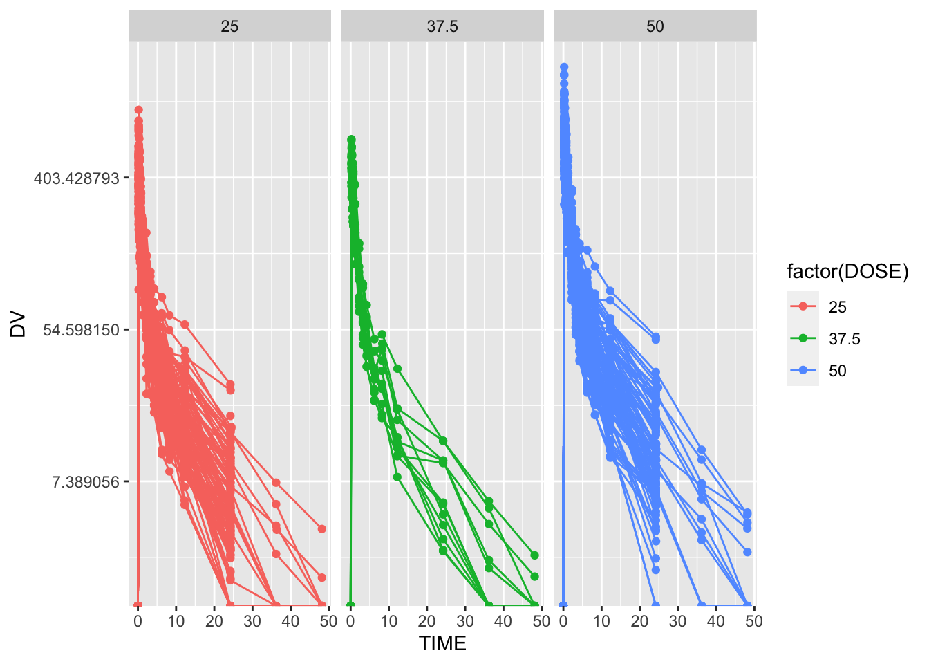
# Save Figure
figure_file = here("fitting-exercise", "figures", "time_series.png")
ggsave(filename = figure_file, plot=plot) 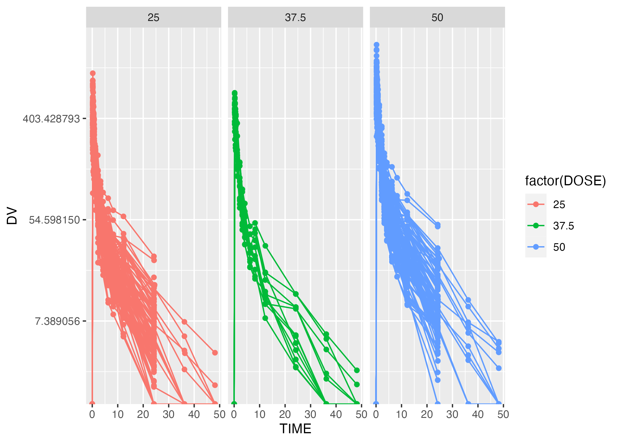
Clearly, there is quite a bit of heterogeneity in these time series, through each tends to trend down more-or-less exponentially (though it seems the rate of decay is decreasing with time.) As indicated here, it appears that some indiciduals received the drug more than once, indicated by having both entries with OCC = 1 and OCC = 2. We will only be considering one dataset for each individual, and we will thus be keeping only 1 adminsitration, that is, OCC = 1.
Task 2: Filtering for observations with OCC = 1 only
The following code chunk removes all observations where OCC = 2. In all fairness, I am not removing OCC = 2 observations overtly. Instead, I am ensuring that I only keep OCC = 1 observations. This way, if we were to update the dataset with more observations from participants who received the drug a third or, even, a fourth time, we would only be analyzing one standard dataset across all participants.
#filter dataframe for observations after first administration of mavoglurant only
mavoglurant_data = mavoglurant_data %>%
  dplyr::filter(OCC == 1) # keep OCC = 1 observations

#note that I am trying to get into the habit of referencing a package each time I use a function derived from it, i.e dplyr::filter(). It's a challenge to remember to do so, but it will be worth it!
Task 3: Isolating \(T_0\) observations and summing total DV for each participant
We would like to compute the total amount of drug (delivered?) for each participant by summing the DV values for each time series.
DV is a measurment of drug concentration (presumably, drug in system, or drug delivered?). Because we are not going to use some sophisticated way of integrating to find the total drug amount (which makes me think this is total amount administered, but could also mean total amount in the blood over time), and instead we are going to sum DV over time, I’d like to get a sense of how much the length of the time series vary. If they vary dramatically, we should consider this when we draw conclusions based on total integrated DV.
The code chunk below generates a boxplot to compare the lengths of time series collected for participants, stratified by the dosage received.
#list to store time series lengths by dose
series_lengths = list()
for(i in 1:length(levels(factor(mavoglurant_data$DOSE)))){

  lengths = mavoglurant_data %>%
    filter(DOSE == levels(factor(mavoglurant_data$DOSE))[i]) %>%
    group_by(ID) %>%
    count() %>%
    pull(n)

  series_lengths[[i]] = lengths
}

df = data.frame(lengths = c(series_lengths[[1]], series_lengths[[2]], series_lengths[[3]]),
                dose = c(rep("25", length(series_lengths[[1]])), rep("37.5", length(series_lengths[[2]])), rep("50", length(series_lengths[[3]]))))

plot = ggplot() + geom_boxplot(data = df, aes(x = dose, y = lengths, fill = factor(dose))) #filling in boxplots looks cooler than outlining htem, in my opinion!

# Save Figure
figure_file = here("fitting-exercise", "figures", "time_series_lengthsbydose.png")
ggsave(filename = figure_file, plot=plot) 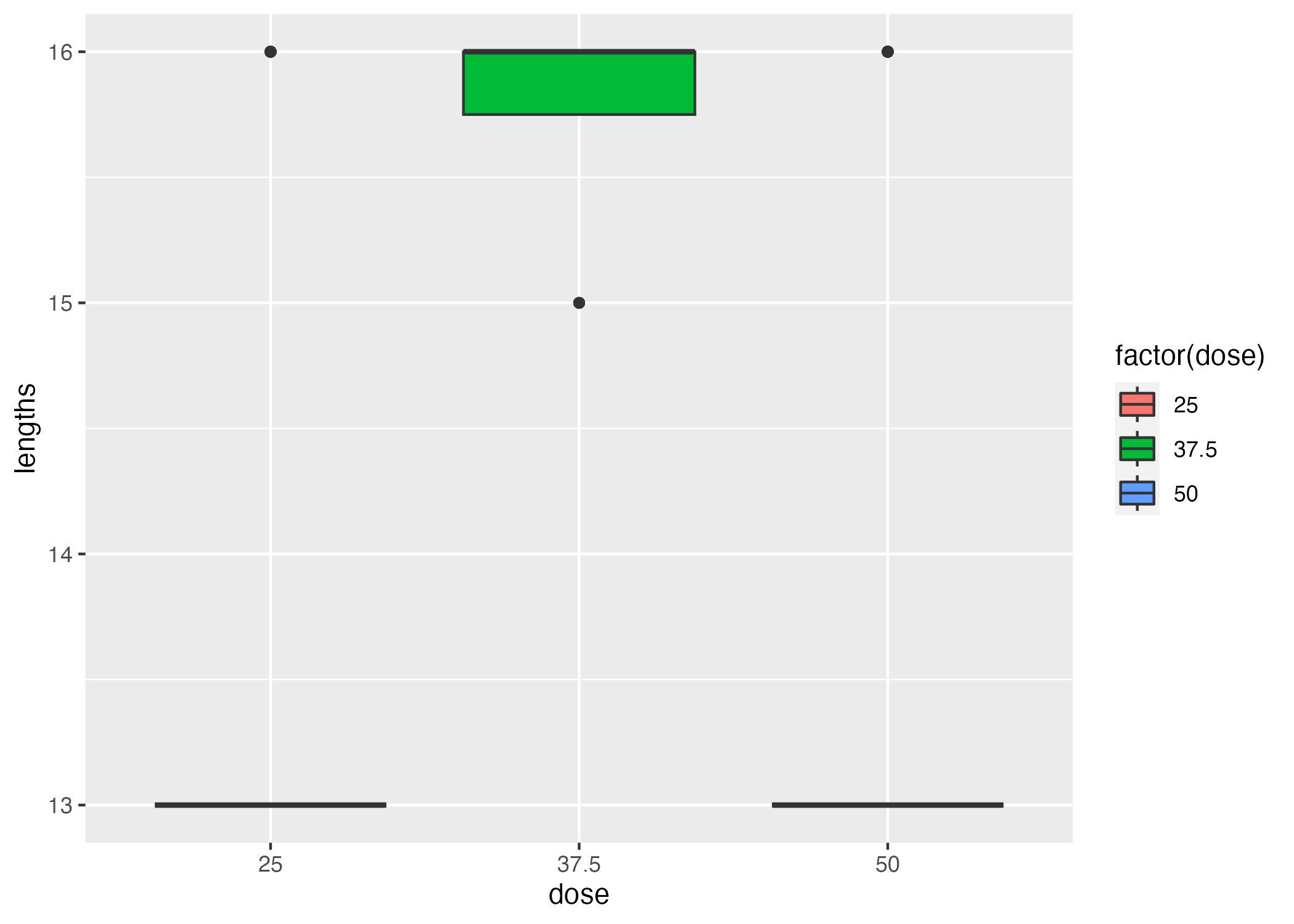
From Figure 2, it appears that time series collected for participants given a dose of 37.5 tend to be longer than the time series collected for participants given the other two dosages. However, the mean difference is 3 time points. If these time points occur later in the time series, when DV is significantly lower than the initial DV (Figure 1), the difference in the sum of DV values may not be too extreme; however, if these were to occur earlier in the time series compared to the other two dosages, when concentrations are high, then we’ve a reason to worry. This applies to the distribution of points collected at different times after original dose delivery, as well - if time series are long but all observations were made at a significantly longer time elapsed from time 0, then we’d have an artificially low sum. We are not going to address this issue moving forward (i.e by fitting to some function and integrating the model function under the length of the series), but I think it is particularly important to have a more visual and intuitive understanding of the issue.
Perhaps I’ll revisit this after the model fitting portion of our exercise…
The code chunk below calculates the sum of DV values for each time series collected for each dosage and stores these sums in a data frame object named sums_nonzero; the “nonzero” nomer distinguishes the dataframe on the basis that all initial TIME == 0 measurements are disregarded and not included in the sum.
For completeness, we also create a data frame of all initial observations, named t0_obs.
We join these together to generate a dataframe of size 120 x 18, which we will call mavoglurant_data_cleaned. In our sums_nonzero dataframe, we have one observation per ID, where a row lists the sum total DV across all time series points (excluding TIME == 0) for an ID. We also have one observation per ID in our t0_obs dataframe, which contains the initial TIME == 0 DV observation and other defining characteristics of this first observation for each participant ID. We can use left_join(), with ID as our primary key, to join these dataframes.
# excluding observations with TIME == 0 and summing all DV per ID
sums_nonzero = mavoglurant_data %>%
  filter(TIME != 0) %>%
  summarize(y = sum(DV), .by = ID)

# including only TIME == 0
t0_obs = mavoglurant_data %>%
  filter(TIME == 0)

# join the dfs
mavoglurant_data_cleaned = left_join(t0_obs, sums_nonzero, by = "ID")
Task 4: Cleaning joined dataframe
Lastly, we want to remove unnecessary variables from the joined dataframe mavoglurant_data_cleaned and convert categorical variables to type factor.
The code chunk below selects the Y, DOSE, AGE, SEX, RACE, RATE, WT, and HT variables, and treats SEX and RACE as factors.
#finish cleaning df
mavoglurant_data_cleaned = mavoglurant_data_cleaned %>%
  select(y, DOSE, RATE, AGE, SEX, RACE, WT, HT) %>%
  mutate(SEX = factor(SEX), RACE = factor(RACE))

#write to an rds file
# save summary tables
data_file = here("ml-models-exercise", "data", "mavoglurant_data_cleaned.rds")
saveRDS(mavoglurant_data_cleaned, file = data_file)
Model Fitting: continuous outcomes
DOSE as a predictor of y
Here, we know that y is the sum of our DV values after TIME==0 for a time series. We also know that DV is related to drug concentration. So, we can already anticipate there will be some relationship between the initial DOSE and y.
The DOSE variable is categorical and the y variable is continuous, so I will try to visualize this anticipated relationship by plotting a boxplot of y for each DOSE.
# plot
plot = ggplot() + geom_boxplot(data = mavoglurant_data_cleaned, aes(x = factor(DOSE), y = y, fill = factor(DOSE))) + geom_point(data = mavoglurant_data_cleaned, aes(x = factor(DOSE), y = y)) + labs(x = "Dose", y = "DV at Time 0")

plot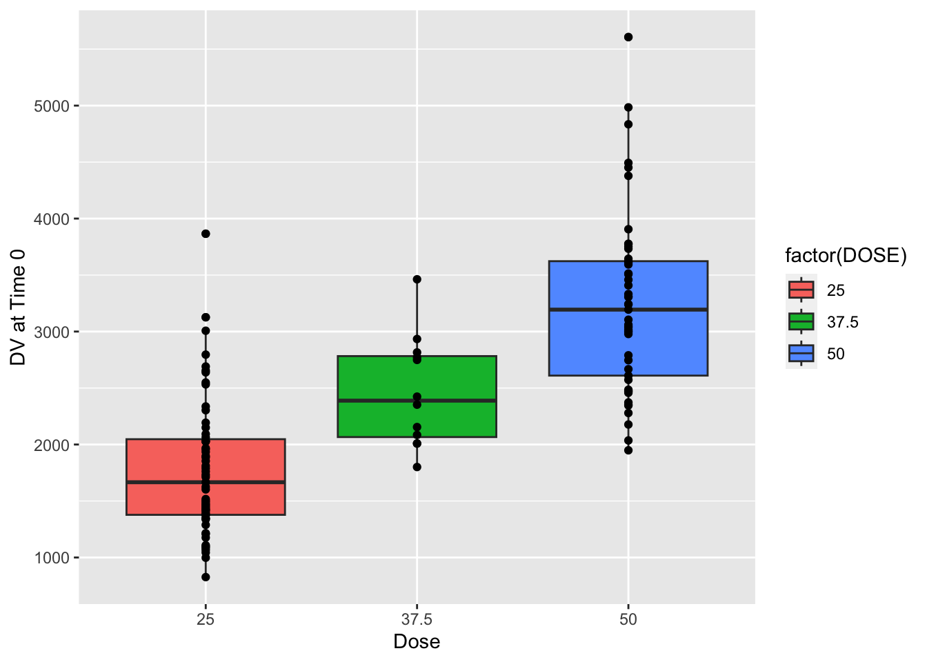
Clearly, y appears to increase with DOSE. However, there is significant overlap between the points. While we can anticipate this trend is significant, we still have two goals for our model:
- Can we parameterize the dependence of
yonDOSEwith some GLM (we can use a linear model)? - How significant is this relationship (we can use ANOVA on our linear model)?
We would like to find a linear model to describe the relationship between y and DOSE, and we are fine to begin our fitting by looking for ordinary least squares. Thus, our model will take the form y ~ DOSE, will be linear with categorical predictor for continuous outcome, and we are fine with the lm method.
We can test whether the mean y predicted by DOSE is significantly different by dosage using ANOVA.
### fitting a linear model
# define recipe with recipes package
rec_y_DOSE <-
  recipes::recipe(y ~ DOSE,
         data = mavoglurant_data_cleaned)

# choose model with parsnip package
y_DOSE_reg =
  parsnip::linear_reg() %>% #linear regression model
  parsnip::set_engine("lm") %>% #with lm method
  parsnip::set_mode("regression") #mode = regression, mode outcome is numeric

# we can turn this into a workflow with workflows package
y_DOSE_reg_WF =
  workflows::workflow() %>% #defining workflow object
  workflows::add_model(y_DOSE_reg) %>% #choosing the model for the workflow
  workflows::add_recipe(rec_y_DOSE) #adding the recipe - which variables for outcome, predictor, any interactions...

# fitting the model with fit()
y_DOSE_reg_model = fit(y_DOSE_reg_WF, data = mavoglurant_data_cleaned)
table1 = y_DOSE_reg_model %>% tidy()


### Testing if the mean ys are significantly different
# ANOVA
anova_y_DOSE_reg = y_DOSE_reg_model %>% extract_fit_engine() %>% anova()
table2 = anova_y_DOSE_reg %>% tidy()

### saving table results
# save summary tables
summarytable_file = here("fitting-exercise", "tables", "y_DOSE_reg.rds")
saveRDS(table1, file = summarytable_file)

summarytable_file = here("fitting-exercise", "tables", "anova_y_DOSE_reg.rds")
saveRDS(table2, file = summarytable_file)| term | estimate | std.error | statistic | p.value |
|---|---|---|---|---|
| (Intercept) | 323.06249 | 199.048513 | 1.623034 | 0.1072508 |
| DOSE | 58.21289 | 5.193797 | 11.208155 | 0.0000000 |
The output of tidymodel’s fit() on our linear regression by lm model provides our estimated parameters (“estimate”, Table 1), as well as the standard error (\(\sigma / \sqrt{n}\)). Before we examine the results of our ANOVA, however, we want to take a closer look at the fit of the linear model we fed into the analysis. Below, we use the yardstick package to determine the root mean squared error and correlation coefficient of the linear regression between y and DOSE.
# calculate r^2 and RMSE from y_DOSE_reg model
## make predictions based on real DOSE observations
predictions_y_DOSE_reg = data.frame(predictor = mavoglurant_data_cleaned$DOSE,
                                    .pred = predict(y_DOSE_reg_model, new_data = mavoglurant_data_cleaned %>% select(-y)), #use regression model to make y predictions from existing DOSE observations
                                    observation = mavoglurant_data_cleaned$y) #bind to observed y observations

## lets take a look
plot = ggplot() + geom_point(data = predictions_y_DOSE_reg, aes(x = predictor, y = observation, color = factor(predictor))) +
          geom_point(data = predictions_y_DOSE_reg, aes(x = predictor, y = .pred)) +
          geom_line(data = predictions_y_DOSE_reg, aes(x = predictor, y = .pred), linetype = "dashed") +
          labs(x = "Dose", y = "DV sum", title = "Regression model prediction of DV sum by dose")

## now lets calculate our metrics
metrics = yardstick::metric_set(rmse, rsq)
table = metrics(predictions_y_DOSE_reg, truth = observation, estimate = .pred)

## add rmse and rsq to plot
plot = plot + annotate("text", y = 5000, x = 32.5, label = paste0("RMSE = ", round(table[1,3], 0), "\n rsq = ", round(table[2,3], 3)))

# saving outputs
summarytable_file = here("fitting-exercise", "tables", "metrics_y_DOSE_reg.rds")
saveRDS(table, file = summarytable_file)

figure_file = here("fitting-exercise", "figures", "metrics_y_DOSE_reg.png")
ggsave(filename = figure_file, plot=plot) 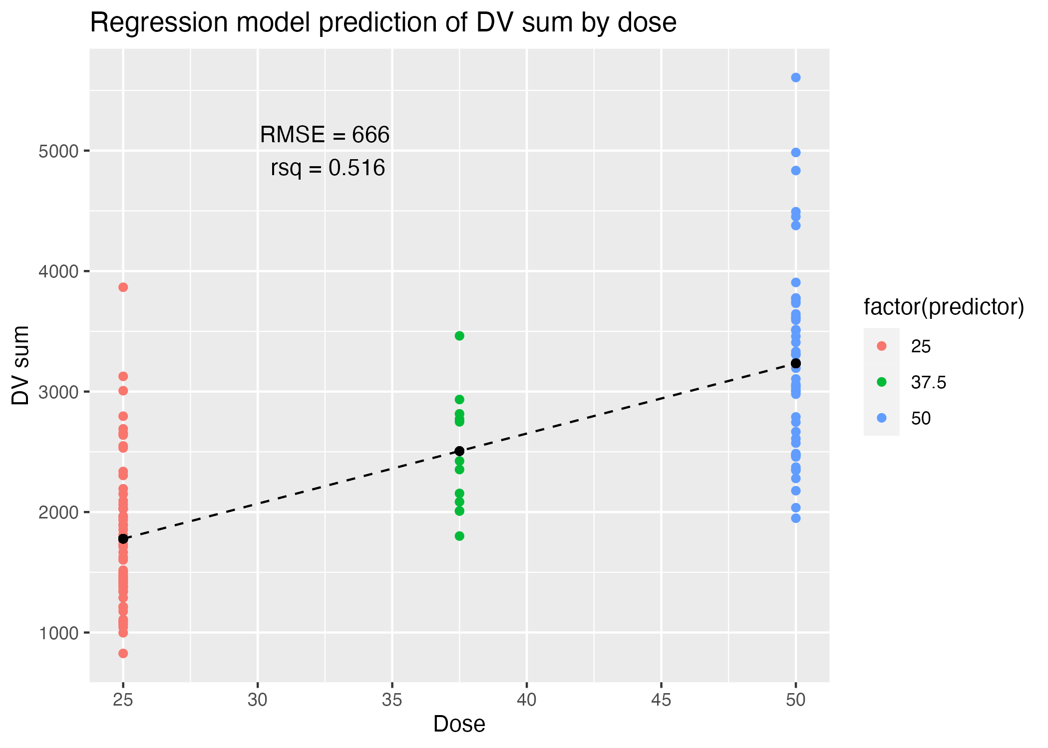
| .metric | .estimator | .estimate |
|---|---|---|
| rmse | standard | 666.4617870 |
| rsq | standard | 0.5156446 |
Clearly, we can see that the linear regression captured some linear relationship between dose and the sum total DV, y. There is clearly quite a bit of variance among the observed values around the estimate predicted by our linear model for each dose (colored vs black points, Figure 3), and similarly, our model fit displays quite a high RMSE (666) and low \(r^2\) (0.516).
The ANOVA does reveal that the differences in estimates from the regression model are significant, with a p-value of 2.6931057^{-20}. Let’s see if we can capture a better model by utilizing more variables as predictors.
| term | df | sumsq | meansq | statistic | p.value |
|---|---|---|---|---|---|
| DOSE | 1 | 56743749 | 56743749.1 | 125.6227 | 0 |
| Residuals | 118 | 53300558 | 451699.6 | NA | NA |
DOSE, RATE, AGE, SEX, RACE, HT, and WT as predictors of y
We’ve demonstrated that dose correlates positively with the sum total DV y; we’ve also demonstrated that there is quite a bit of heterogeneity around the estimate predicted by DOSE alone. Here, we would like to discern whether a model utilizing DOSE, RATE, AGE, SEX, RACE, HT, and WT all as predictors of y will provide a better fitting model. This will ultimately raise the question of whether we are overfitting by introducing too many parameters, but let’s not get ahead of ourselves!
The questions addressed in this section are as follows:
- Can we parameterize the dependence of
yonDOSE,RATE,AGE,SEX,RACE,HT, andWTwith some GLM (we can use a linear model)? - How do the RMSE and \(r^2\) of this model compare to our previous
y ~ DOSEregression?
### fitting a linear model
# define recipe with recipes package
rec_y_all <-
  recipes::recipe(y ~ DOSE + RATE + AGE + SEX + RACE + WT + HT,
         data = mavoglurant_data_cleaned)

# choose model with parsnip package
y_all_reg =
  parsnip::linear_reg() %>% #linear regression model
  parsnip::set_engine("lm") %>% #with lm method
  parsnip::set_mode("regression") #mode = regression, mode outcome is numeric

# we can turn this into a workflow with workflows package
y_all_reg_WF =
  workflows::workflow() %>% #defining workflow object
  workflows::add_model(y_all_reg) %>% #choosing the model for the workflow
  workflows::add_recipe(rec_y_all) #adding the recipe - which variables for outcome, predictor, any interactions...

# fitting the model with fit()
y_all_reg_model = fit(y_all_reg_WF, data = mavoglurant_data_cleaned)
table1 = y_all_reg_model %>% tidy()

### saving table results
# save summary tables
summarytable_file = here("fitting-exercise", "tables", "y_all_reg.rds")
saveRDS(table1, file = summarytable_file)| term | estimate | std.error | statistic | p.value |
|---|---|---|---|---|
| (Intercept) | 3399.953281 | 1819.271104 | 1.8688547 | 0.0643032 |
| DOSE | 146.874595 | 50.861892 | 2.8877139 | 0.0046733 |
| RATE | -14.354042 | 8.359358 | -1.7171225 | 0.0887711 |
| AGE | 1.777301 | 7.798316 | 0.2279083 | 0.8201406 |
| SEX2 | -338.676786 | 215.335328 | -1.5727878 | 0.1186399 |
| RACE2 | 125.040505 | 128.703178 | 0.9715417 | 0.3334101 |
| RACE7 | -398.431716 | 444.324300 | -0.8967138 | 0.3718300 |
| RACE88 | -69.064910 | 242.717190 | -0.2845489 | 0.7765248 |
| WT | -23.703602 | 6.351282 | -3.7320972 | 0.0003023 |
| HT | -717.053335 | 1094.568090 | -0.6551016 | 0.5137700 |
Clearly, DOSE, RATE, and WT are significant predictors of the sum total DV (Table 4).
However, when we observe our metrics:
# calculate r^2 and RMSE from y_DOSE_reg model
## make predictions based on real DOSE observations
predictions_y_all_reg = data.frame(predictor_1= mavoglurant_data_cleaned$DOSE,
                                   .pred = predict(y_all_reg_model, new_data = mavoglurant_data_cleaned %>% select(-y)), #use regression model to make y predictions from existing observations
                                   observation = mavoglurant_data_cleaned$y) #bind to observed y observations

## lets take a look
plot = ggplot() + geom_point(data = predictions_y_all_reg, aes(x = observation, y = .pred, color = factor(predictor_1))) +
          geom_abline(linetype = "dashed") +
          labs(x = "Observed", y = "Predicted", title = "DV sums observed and predicted by regression")

## now lets calculate our metrics
metrics = yardstick::metric_set(rmse, rsq)
table = metrics(predictions_y_all_reg, truth = observation, estimate = .pred)

## add rmse and rsq to plot
plot = plot + annotate("text", y = 5000, x = 2000, label = paste0("RMSE = ", round(table[1,3], 0), "\n rsq = ", round(table[2,3], 3)))

# saving outputs
summarytable_file = here("fitting-exercise", "tables", "metrics_y_all_reg.rds")
saveRDS(table, file = summarytable_file)

figure_file = here("fitting-exercise", "figures", "metrics_y_all_reg.png")
ggsave(filename = figure_file, plot=plot) 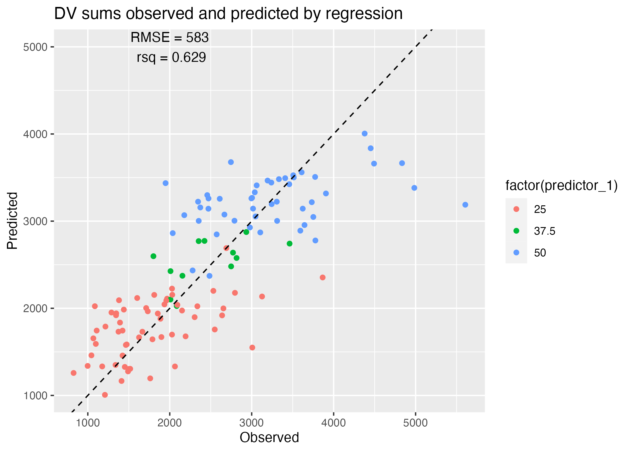
| .metric | .estimator | .estimate |
|---|---|---|
| rmse | standard | 583.0903868 |
| rsq | standard | 0.6292464 |
Table 5 reveals that a model utilizing all variables as predictors of total DV sums does a slightly better job at recapitulating our observed y values, explaining 63% of the variance as opposed to the 52% explained by DOSE alone. However, if we were to penalize for the number of predictors and parameters, I’m not sure we’d agree that this model is the better-fitting! Once again, this depends on our goal - do we wish to reproduce our observations with the greatest accuracy? If we were to sample smaller subsets of our data and refit, would we still be able to reproduce all of our results with the same accuracy, and how much variance would we observe in the estimated parameters of each iteration?
Model fitting: categorical outcome
Previously, we formulated two linear models to predict the continuous outcome of the sum total DV for each time series, which we called y, with either initial drug DOSE alone or all predictor variables as predictors. This led us to ask an interesting question: do we care the most about accuracy, precision, and/or biological meaning in our model?
Here, we would like to ask a similar question: can we accurately predict the sex of an individual based upon the dosage of the drug they recieved? If we fit a model with all of their other characteristic variables, will we see a greater fit, and will this greater fit be meaningful enough that we would opt for the more parameterized model?
Here, SEX is a categorical variable we intend to predict; as such, we can use a logistic model. We will be using the default threshold of 0.5 as a cutoff to categorize our participants as eitherSEX == 1, or “success” (so it’s probably women ;)), or SEX == 2, or failure.
Predicting SEX by DOSE
Here, we’d like to see how well we can fit a logistic model to SEX by the predictor DOSE; perhaps certain dosages are more frequently assigned to one sex than the other? SEX is a binary categorical variable, and DOSE is a categorical variable with more than two levels. We will thus use a logistic regression to classify observations into either SEX category, 0 or 1.
The logistic regression estimates 2 parameters to produce a steep sigmoidal probability of one category of a binary categorical variable and some continuous predictor ( or some probability of success based on categorical predictors). The two parameters produce a sigmoidal relationship by assuming the odds of success increase multiplicatively for some unit increase in the predictor (that is, the natural log of the odds function of success is linear). For myself and others, a wonderful resource explaining the inutition behind this can be found in this online chapter.
If the predictor is continuous, we’d see something along the lines (ha, pun intended) of Figure 5:
### fitting a linear model
# define recipe with recipes package
recipe <-
  recipes::recipe(SEX ~ HT,
         data = mavoglurant_data_cleaned)

# choose model with parsnip package
reg =
  parsnip::logistic_reg() %>% #linear regression model
  parsnip::set_engine("glm") %>% #with glm method - which we cant use lm for a logistic model becuase OLS-like statstics don't make much sense here!
  parsnip::set_mode("classification") #mode = classification, mode outcome is categorical

# we can turn this into a workflow with workflows package
reg_WF =
  workflows::workflow() %>% #defining workflow object
  workflows::add_model(reg) %>% #choosing the model for the workflow
  workflows::add_recipe(recipe) #adding the recipe - which variables for outcome, predictor, any interactions...

reg_model = fit(reg_WF, data = mavoglurant_data_cleaned)
table1 = reg_model %>% tidy()

###plot
plot = ggplot() + geom_point(data = mavoglurant_data_cleaned, aes(x = HT, y = (as.numeric(SEX))-1)) +
  stat_function(fun = function(x) exp(table1$estimate[1] + table1$estimate[2]*x)/(1+exp(table1$estimate[1] + table1$estimate[2]*x))) +
  labs(x = "HT", y = "probability of Sex 2", title = "Example Logistic Regression")

###save fig
figure_file = here("fitting-exercise", "figures", "logistic_example.png")
ggsave(filename = figure_file, plot=plot) 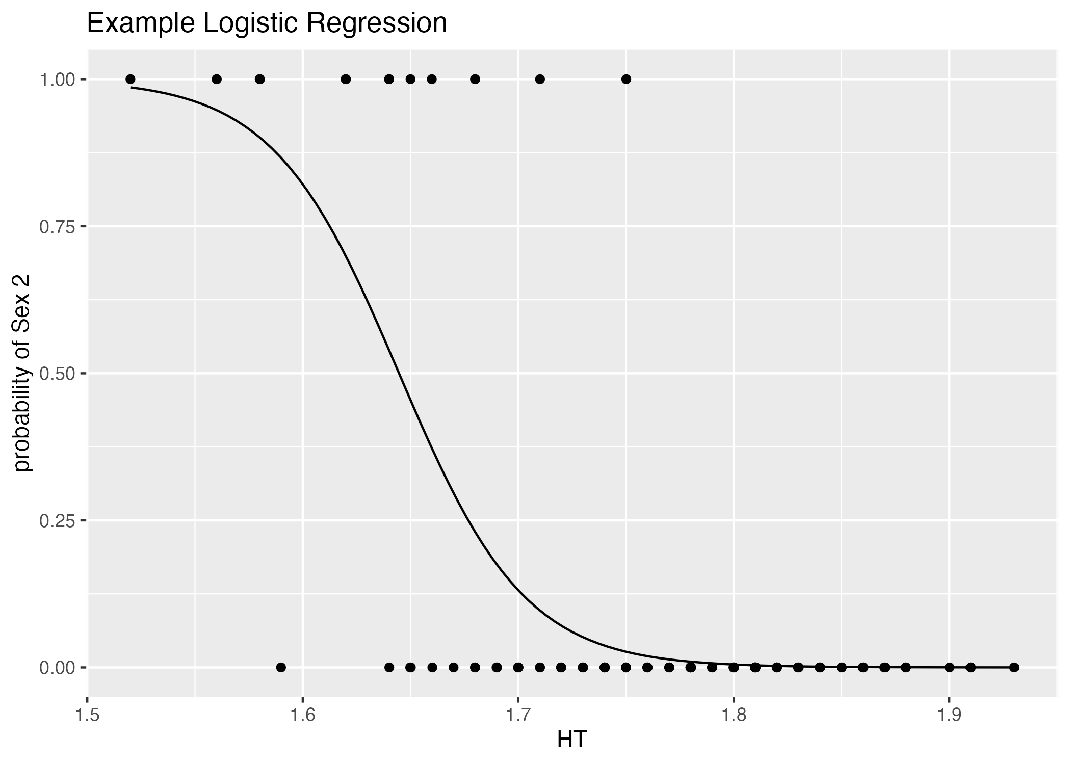
Note that we can also perform a logistic regression utilizing a categorical predictor - and, here, we can treat DOSE as a categorical variable or a numeric variable. I will be treating it numerically, because increasing dosage can have biological significance which may be indicated by sexual dimorphism!
Here, we are preforming a logistic regression to predict the probability of belonging to SEX category 2 based on the variable DOSE. Our formula will be SEX ~ DOSE, we will use a logistic_reg() model with an glm “engine”, and the mode of our model is classification as the output variable is categorical.
### fitting a linear model

# define recipe with recipes package
recipe <-
  recipes::recipe(SEX ~ DOSE,
         data = mavoglurant_data_cleaned)

# choose model with parsnip package
reg =
  parsnip::logistic_reg() %>% #linear regression model
  parsnip::set_engine("glm") %>% #with glm method - which we cant use lm for a logistic model becuase OLS-like statstics don't make much sense here!
  parsnip::set_mode("classification") #mode = classification, mode outcome is categorical

# we can turn this into a workflow with workflows package
reg_WF =
  workflows::workflow() %>% #defining workflow object
  workflows::add_model(reg) %>% #choosing the model for the workflow
  workflows::add_recipe(recipe) #adding the recipe - which variables for outcome, predictor, any interactions...

reg_model = fit(reg_WF, data = mavoglurant_data_cleaned)
table1 = reg_model %>% tidy()

###plot
plot = ggplot() + geom_point(data = mavoglurant_data_cleaned, aes(x = DOSE, y = (as.numeric(SEX))-1, color = SEX), alpha = 0.25) +
  stat_function(fun = function(x) exp(table1$estimate[1] + table1$estimate[2]*x)/(1+exp(table1$estimate[1] + table1$estimate[2]*x))) +
  labs(x = "DOSE", y = "probability of Sex 2", title = "Logistic Regression of Sex 2 Prob by Dose")

### saving table results
# save summary tables
summarytable_file = here("fitting-exercise", "tables", "SEX_DOSE_reg.rds")
saveRDS(table1, file = summarytable_file)

###save fig
figure_file = here("fitting-exercise", "figures", "logistic_sex_dose.png")
ggsave(filename = figure_file, plot=plot) 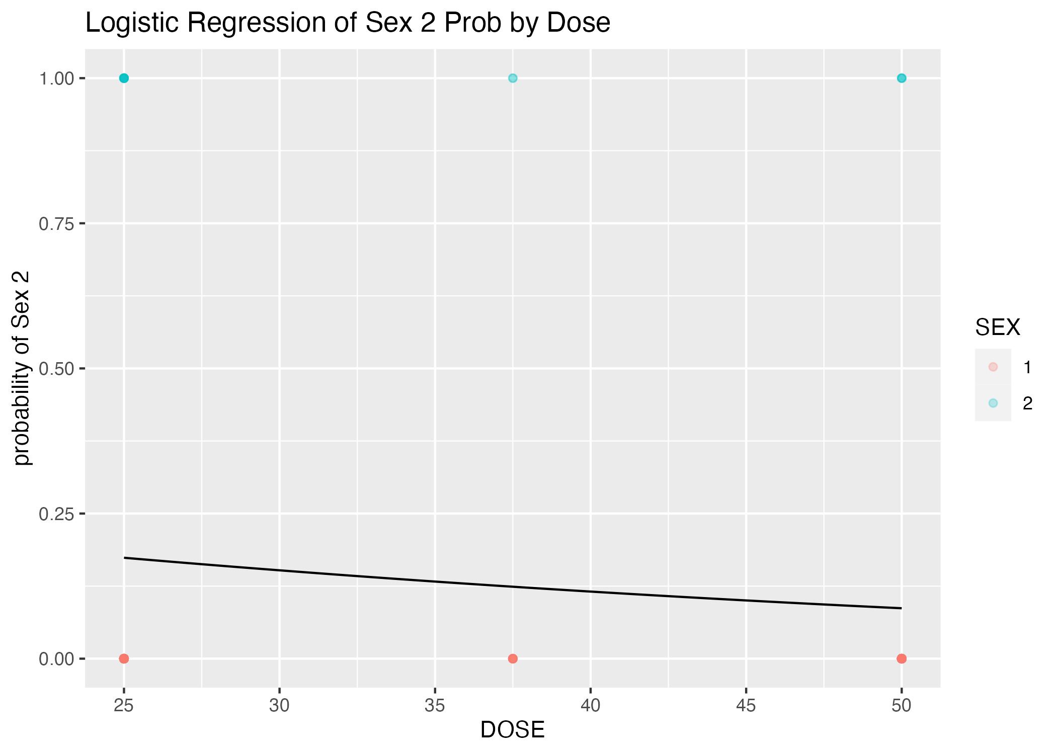
| term | estimate | std.error | statistic | p.value |
|---|---|---|---|---|
| (Intercept) | -0.7648181 | 0.8539475 | -0.8956266 | 0.3704522 |
| DOSE | -0.0317544 | 0.0243205 | -1.3056660 | 0.1916662 |
Evidently, DOSE is a pretty poor predictor (say that five times fast) of SEX (see p.values for parameter estimates, Table 6). This is certainly not helped by the potential that SEX category 1 is over-represented in the dataset (see opacity of points, Figure 6). (Perhaps mavolglurant is a drug used more by one sex than the other?)
# calculate r^2 and RMSE from y_DOSE_reg model
## make predictions based on real DOSE observations
predictions = data.frame(predictor = mavoglurant_data_cleaned$DOSE,
                                    .pred = predict(reg_model, new_data = mavoglurant_data_cleaned %>% select(-SEX)), #use regression model to make SEX predictions from existing DOSE observations
                                    observation = mavoglurant_data_cleaned$SEX) #bind to observed sex observations
#plot barplot
plot = predictions %>%
  group_by(predictor) %>%
  summarize(obs_succeses = sum(as.numeric(observation)), pred_successes = sum(as.numeric(.pred_class))) %>%
  pivot_longer(cols = c("obs_succeses", "pred_successes"),
               names_to = "data",
               values_to = "SEX2_Count") %>%
  ggplot(aes(x = as.factor(predictor), y = SEX2_Count, fill = data)) + geom_bar(stat = "identity", position = position_dodge()) + labs(x = "DOSE", y = "Count of Sex 2 participants")


## now lets calculate our metrics
### accuracy
acc = accuracy(predictions, truth = observation, estimate = .pred_class)

### ROC AUC
predictions = data.frame(predictor = mavoglurant_data_cleaned$DOSE,
                                    predict(reg_model, new_data = mavoglurant_data_cleaned %>% select(-SEX), type = "prob"), #use regression model to make SEX predictions from existing DOSE observations, returns probabilities of sex categories (2 cols)
                                    observation = mavoglurant_data_cleaned$SEX) #bind to observed sex observations

rocauc = roc_auc(predictions, truth = observation, .pred_1) #roc with probabiliy of sex 2 thresholds
plot2 = roc_curve(predictions, truth = observation, .pred_1) %>% #plot roc curve
               autoplot() + annotate("text", x = 0.75, y = 0.25, label = paste0("AUC = ", round(rocauc$.estimate, 3)))

## adjust barplot with accuracy metrics
plot = plot + annotate("text", x = "50", y = 60, label = paste0("accuracy = ", round(acc$.estimate, 3)))

#save figures
figure_file = here("fitting-exercise", "figures", "metrics_sex_DOSE_reg.png")
ggsave(filename = figure_file, plot=plot)

figure_file = here("fitting-exercise", "figures", "roc_sex_DOSE_reg.png")
ggsave(filename = figure_file, plot=plot2) 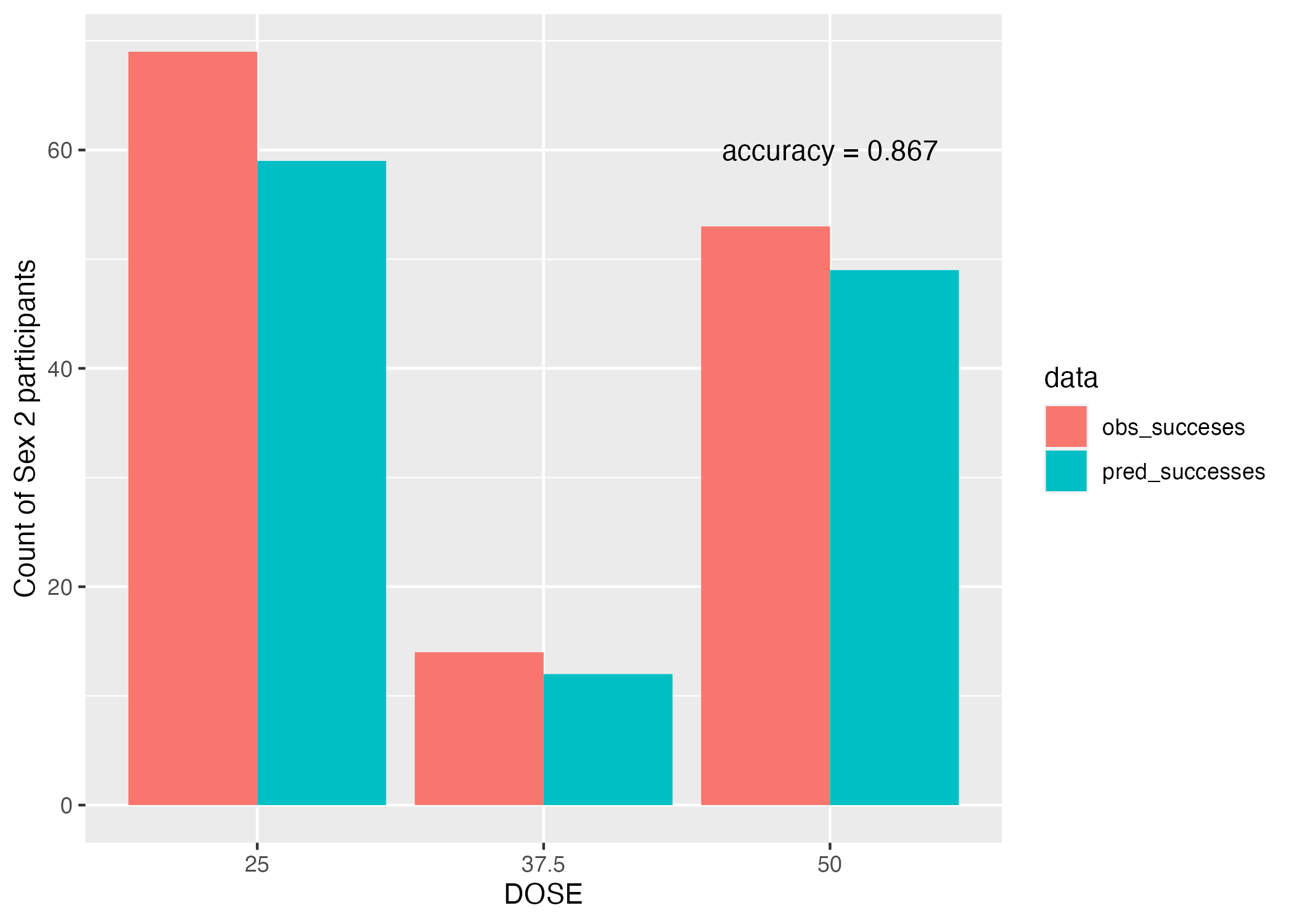
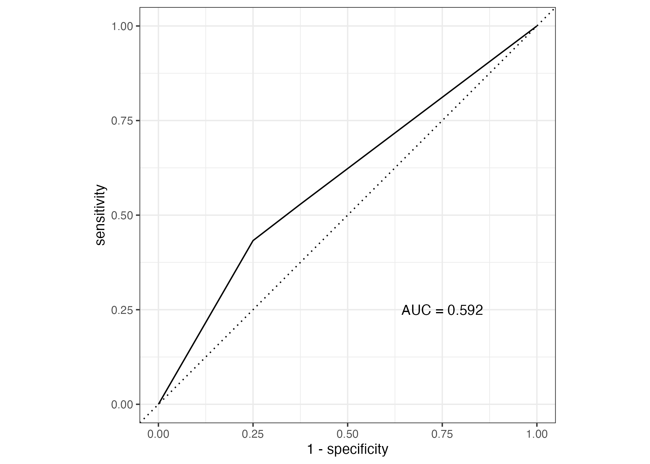
The accuracy is actually pretty high (Figure 7) at 0.867, though our p-value really isn’t.
Predicting SEX by DOSE, RATE, AGE, SEX, RACE, HT, WT, and y.
The code chunk below fits a logistic regression model to predict SEX by the predictors DOSE, RATE, AGE, SEX, RACE, HT, WT, and y.
### fitting a linear model

# define recipe with recipes package
recipe <-
  recipes::recipe(SEX ~ DOSE + RATE + AGE + y + RACE + WT + HT,
         data = mavoglurant_data_cleaned)

# choose model with parsnip package
reg =
  parsnip::logistic_reg() %>% #linear regression model
  parsnip::set_engine("glm") %>% #with glm method - which we cant use lm for a logistic model becuase OLS-like statstics don't make much sense here!
  parsnip::set_mode("classification") #mode = classification, mode outcome is categorical

# we can turn this into a workflow with workflows package
reg_WF =
  workflows::workflow() %>% #defining workflow object
  workflows::add_model(reg) %>% #choosing the model for the workflow
  workflows::add_recipe(recipe) #adding the recipe - which variables for outcome, predictor, any interactions...

reg_model = fit(reg_WF, data = mavoglurant_data_cleaned)
table1 = reg_model %>% tidy()

###plot
plot = ggplot() + geom_point(data = mavoglurant_data_cleaned, aes(x = HT, y = (as.numeric(SEX))-1, color = AGE, shape = RACE)) +
  stat_function(fun = function(x) exp(table1$estimate[1] + table1$estimate[10]*x)/(1+exp(table1$estimate[1] + table1$estimate[10]*x))) +
  labs(x = "HT", y = "probability of Sex 2", title = "Logistic Regression, Probability of Sex 2 by all descriptors")

### saving table results
# save summary tables
summarytable_file = here("fitting-exercise", "tables", "SEX_all_reg.rds")
saveRDS(table1, file = summarytable_file)

###save fig
figure_file = here("fitting-exercise", "figures", "logistic_sex_all.png")
ggsave(filename = figure_file, plot=plot) 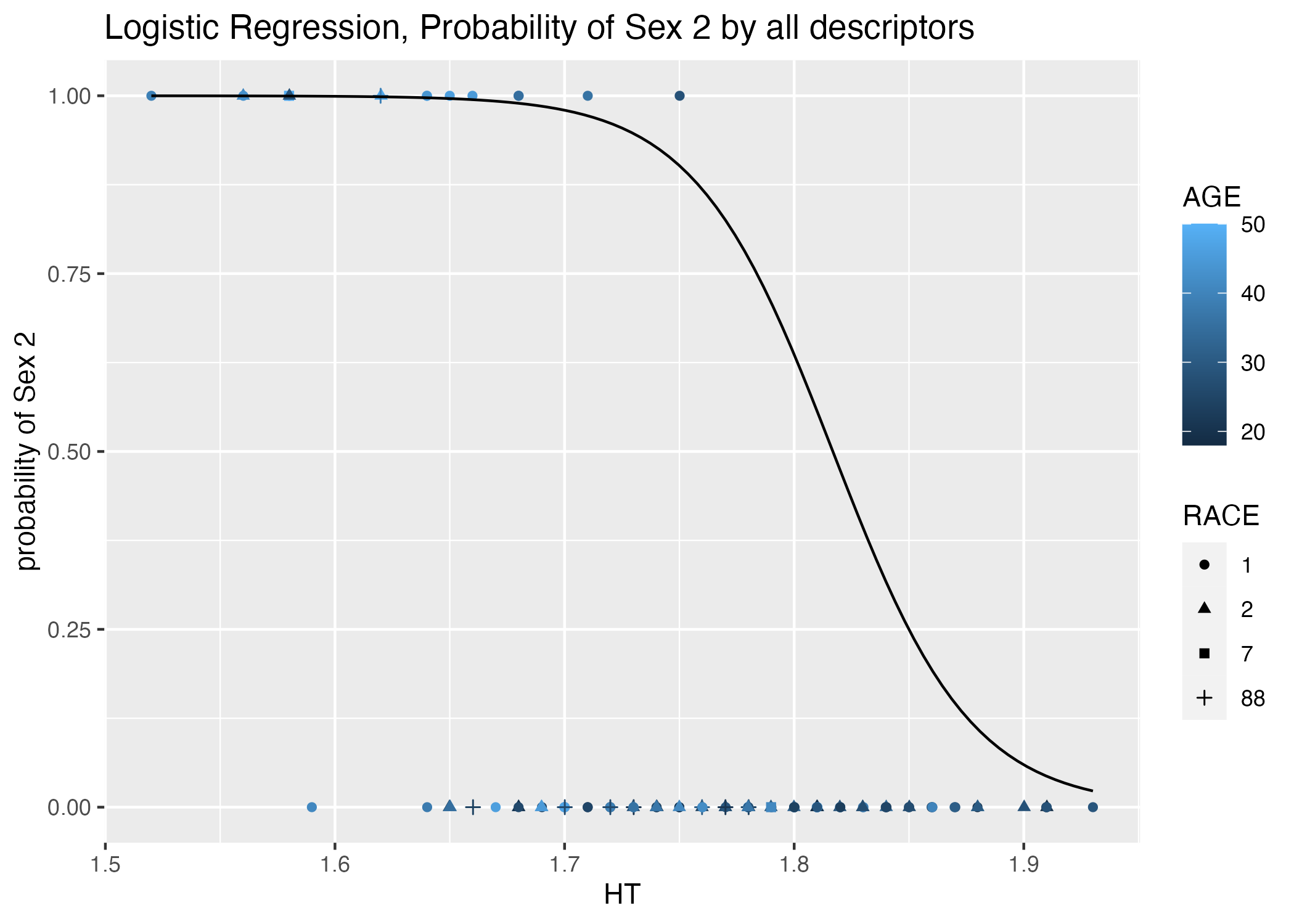
mavoglurant_data_cleaned dataframe. Point color indicates age, while point shape indicates race category. The regression line for continuous predictor height is plotted.| term | estimate | std.error | statistic | p.value |
|---|---|---|---|---|
| (Intercept) | 60.2826915 | 18.0502582 | 3.3397135 | 0.0008386 |
| DOSE | -0.8490976 | 191.9637237 | -0.0044232 | 0.9964708 |
| RATE | 0.1363655 | 31.9939454 | 0.0042622 | 0.9965992 |
| AGE | 0.0834182 | 0.0607202 | 1.3738127 | 0.1694998 |
| y | -0.0010377 | 0.0009642 | -1.0763124 | 0.2817876 |
| RACE2 | -1.9240578 | 1.3759139 | -1.3983854 | 0.1619974 |
| RACE7 | 0.1185532 | 3.8410314 | 0.0308649 | 0.9753773 |
| RACE88 | -1.4978163 | 2.1944584 | -0.6825449 | 0.4948945 |
| WT | -0.0626504 | 0.0794790 | -0.7882638 | 0.4305424 |
| HT | -33.1798562 | 11.0835782 | -2.9936051 | 0.0027570 |
The best predictors of of SEX appear to be HT, Race, AGE, and potentially y (Table 7).Dose, y, RACE==32 or 88, WT, and HT are negatively correlated with SEX==2. Biologically, if we consider women to be shorter than men on average, then maybe my choice of SEX == 2 as the “success” variable under the assumption that SEX 2 is women was fortuitous ;).
# calculate r^2 and RMSE from y_DOSE_reg model
## make predictions based on real DOSE observations
predictions = data.frame(predictor = mavoglurant_data_cleaned$HT,
                                    .pred = predict(reg_model, new_data = mavoglurant_data_cleaned %>% select(-SEX)), #use regression model to make SEX predictions from existing DOSE observations
                                    observation = mavoglurant_data_cleaned$SEX) #bind to observed sex observations
#plot barplot
observed_successes = predictions %>% select(predictor, observation) %>% filter(observation==2)
predicted_successes = predictions %>% select(predictor, .pred_class) %>% filter(.pred_class==2)
for_hist = data.frame(HT = c(observed_successes$predictor, predicted_successes$predictor),
                      count = c(rep("observed", nrow(observed_successes)), rep("predicted", nrow(predicted_successes))))

plot = for_hist %>%
  ggplot() + geom_histogram(aes(x = HT, y = ..density.., color = count, fill = count), alpha = 0.25, position = "identity", bins = 20) +
  geom_density(aes(x = HT, y=..density.., color = count, fill = count), position = "identity", alpha = 0.5) +
  labs(x = "HT", y = "density of total SEX == 2 observations", title = "Comparison of classifications of SEX by Logistic regression model against predictor HT")


## now lets calculate our metrics
### accuracy
acc = accuracy(predictions, truth = observation, estimate = .pred_class)

### ROC AUC
predictions = data.frame(predictor = mavoglurant_data_cleaned$HT,
                                    predict(reg_model, new_data = mavoglurant_data_cleaned %>% select(-SEX), type = "prob"), #use regression model to make SEX predictions from existing DOSE observations, returns probabilities of sex categories (2 cols)
                                    observation = mavoglurant_data_cleaned$SEX) #bind to observed sex observations

rocauc = roc_auc(predictions, truth = observation, .pred_1) #roc with probabiliy of sex 2 thresholds
plot2 = roc_curve(predictions, truth = observation, .pred_1) %>% #plot roc curve
               autoplot() + annotate("text", x = 0.75, y = 0.25, label = paste0("AUC = ", round(rocauc$.estimate, 3)))

## adjust barplot with accuracy metrics
plot = plot + annotate("text", x = 1.7, y = 13, label = paste0("accuracy = ", round(acc$.estimate, 3)))

#save figures
figure_file = here("fitting-exercise", "figures", "metrics_sex_all_reg.png")
ggsave(filename = figure_file, plot=plot)

figure_file = here("fitting-exercise", "figures", "roc_sex_all_reg.png")
ggsave(filename = figure_file, plot=plot2) 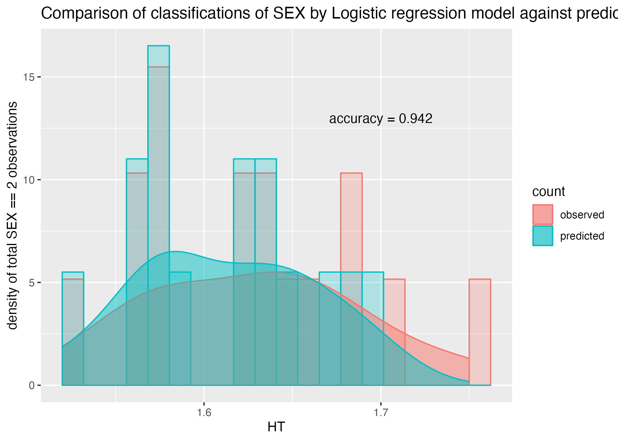
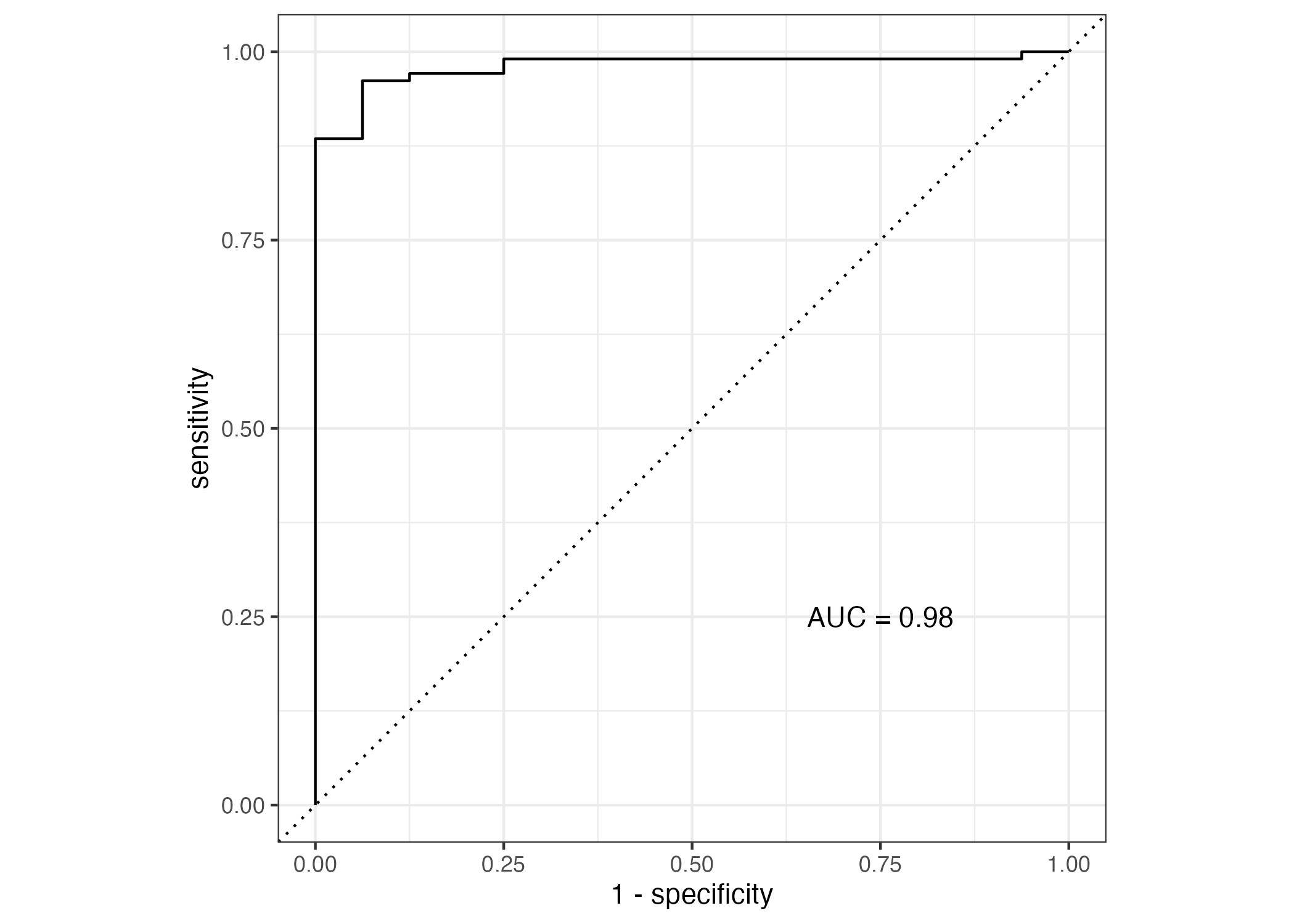
Including more predictors improves the accuracy of the classification model to 94% (Figure 10), and the ROC-AUC performance to 0.98 (Figure 11). This model is certainly better at classification than the previous but, once again, fails to support or predict any biological indicator of SEX by the predictors included in the study and may suffer from fitting with too many unnecessary parameters. We did discover, however, the significance of the contributions of different factors to the prediction of SEX, with HT being the most significant predictor (Table 7). # Model Improvement Assignment
The code chunk below defines the value of a seed, but does not yet set the seed.
rngseed = 1234 #define the number of our seedAs a last step in processing, we know that the RACE factor variable has some bizarre entries (7 or 88), and we are not particularly curious about asking questions regarding this variable now. So, we are going to remove it from the dataset in the code chunk below. I have also kept the RATE variable until this point, but will be removing it for this part of the assessment as well.
mavoglurant_data_cleaned = mavoglurant_data_cleaned %>%
  select(-c(RATE,RACE)) #remove variables RATE and RACE from the cleaned dataset
Now, our dataset mavoglurant_data_cleaned consist of 120 observations of 6 variables: y, DOSE, AGE, SEX, WT, and HT.
In this section, we will be splitting our data into two subsets: a training set and a test set. The training set will be used to fit our models, while the test set will be used to observe whether the fitted model precisely captures the behavior of the data - that is, how well does it perform when predicting the test data? With so few samples, we would ideally perform cross-validation and estimate model performance on unseen data (separate the dat into k staggered subsets, and run through k epochs of training the model on k-1 subsets and testing on the kth subset each epoch.) But, for the sake of learning, we are not going to do that here.
We will be randomly splitting our data 75% into the training set and 25% into the testing set below using the package rsample below:
set.seed(rngseed)
#split the dataset randomly into two sets
banana_split = initial_split(mavoglurant_data_cleaned, prop = 3/4) #prop refers to the proportion in the training set - 75%

# create dataframes for the two sets
training = training(banana_split)
testing = testing(banana_split)
Model Fit Assessment
Here, we fit two linear models to the continuous outcome, y (as a reminder, y is the sum of DV values for a time series). The first utilises DOSE as a predictor, which we anticipate to have some correlation with the total sum of drug concentration measurments over time; the second model utilizes all predictors. Root Mean Squared Error is the metric used to optimize the model. We compare the fit of each model against the fit of a null model, predicting the mean of the observations without predictor variables.
Fitting the models and comparing RMSE metric
The following code chunk utilizes the tidymodels framework to fit a linear regression model (method = lm) with DOSE as a predictor of y:
### fitting a linear model
# define recipe with recipes package
rec_y_DOSE <-
  recipes::recipe(y ~ DOSE,
         data = training)

# choose model with parsnip package
y_DOSE_reg =
  parsnip::linear_reg() %>% #linear regression model
  parsnip::set_engine("lm") %>% #with lm method
  parsnip::set_mode("regression") #mode = regression, mode outcome is numeric

# we can turn this into a workflow with workflows package
y_DOSE_reg_WF =
  workflows::workflow() %>% #defining workflow object
  workflows::add_model(y_DOSE_reg) %>% #choosing the model for the workflow
  workflows::add_recipe(rec_y_DOSE) #adding the recipe - which variables for outcome, predictor, any interactions...

# fitting the model with fit()
train_y_DOSE_reg_model = fit(y_DOSE_reg_WF, data = training)
table1 = y_DOSE_reg_model %>% tidy()

### saving table results
# save summary tables
summarytable_file = here("fitting-exercise", "tables", "y_DOSE_reg_training.rds")
saveRDS(table1, file = summarytable_file)| term | estimate | std.error | statistic | p.value |
|---|---|---|---|---|
| (Intercept) | 323.06249 | 199.048513 | 1.623034 | 0.1072508 |
| DOSE | 58.21289 | 5.193797 | 11.208155 | 0.0000000 |
The output of tidymodel’s fit() on our linear regression by lm model provides our estimated parameters (“estimate”, ?@tbl-y-dose-reg_training), as well as the standard error (\(\sigma / \sqrt{n}\)). Below, we use the yardstick package to determine the root mean squared error and correlation coefficient of the linear regression between y and DOSE.
# calculate r^2 and RMSE from y_DOSE_reg model
## make predictions based on real DOSE observations
predictions_y_DOSE_reg_train = data.frame(predictor = training$DOSE,
                                    .pred = predict(train_y_DOSE_reg_model, new_data = training %>% select(-y)), #use regression model to make y predictions from existing DOSE observations
                                    observation = training$y) #bind to observed y observations

## lets take a look
plot = ggplot() + geom_point(data = predictions_y_DOSE_reg_train, aes(x = predictor, y = observation, color = factor(predictor))) +
          geom_point(data = predictions_y_DOSE_reg_train, aes(x = predictor, y = .pred)) +
          geom_line(data = predictions_y_DOSE_reg_train, aes(x = predictor, y = .pred), linetype = "dashed") +
          labs(x = "Dose", y = "DV sum", title = "Regression model prediction of DV sum by dose")

## now lets calculate our metrics
metrics = yardstick::metric_set(rmse, rsq)
table = metrics(predictions_y_DOSE_reg_train, truth = observation, estimate = .pred)

## add rmse and rsq to plot
plot = plot + annotate("text", y = 4500, x = 32.5, label = paste0("RMSE = ", round(table[1,3], 0), "\n rsq = ", round(table[2,3], 3)))

# saving outputs
summarytable_file = here("fitting-exercise", "tables", "metrics_y_DOSE_reg_training.rds")
saveRDS(table, file = summarytable_file)

figure_file = here("fitting-exercise", "figures", "metrics_y_DOSE_reg_training.png")
ggsave(filename = figure_file, plot=plot) 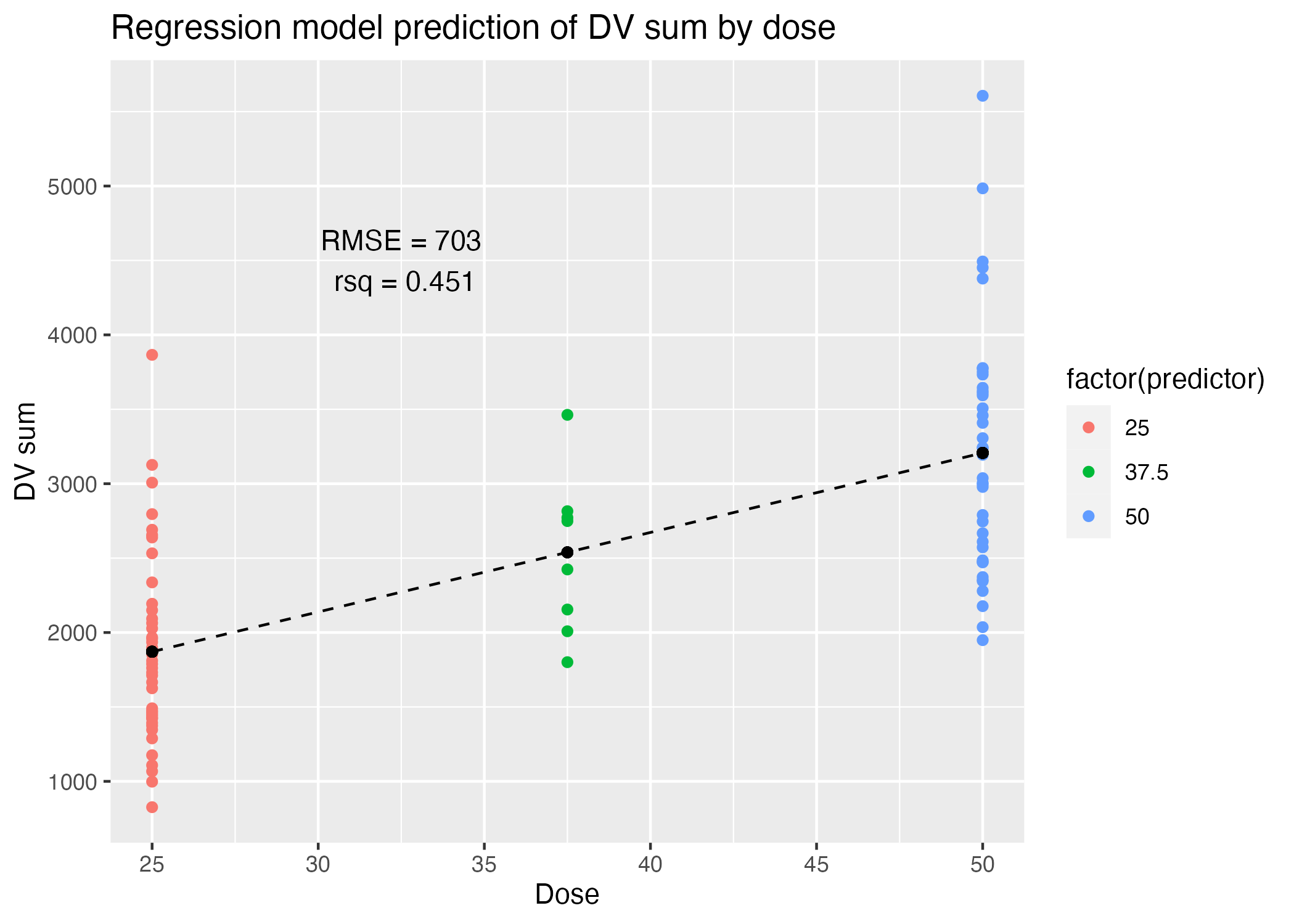
| .metric | .estimator | .estimate |
|---|---|---|
| rmse | standard | 702.8077893 |
| rsq | standard | 0.4507963 |
The following code chunk utilizes the tidymodels framework to fit a multiple linear regression model (method = lm) with all variables as a predictor of y:
### fitting a linear model
# define recipe with recipes package
rec_y_multiple <-
  recipes::recipe(y ~ .,
         data = training)

# choose model with parsnip package
y_multiple_reg =
  parsnip::linear_reg() %>% #linear regression model
  parsnip::set_engine("lm") %>% #with lm method
  parsnip::set_mode("regression") #mode = regression, mode outcome is numeric

# we can turn this into a workflow with workflows package
y_multiple_reg_WF =
  workflows::workflow() %>% #defining workflow object
  workflows::add_model(y_multiple_reg) %>% #choosing the model for the workflow
  workflows::add_recipe(rec_y_multiple) #adding the recipe - which variables for outcome, predictor, any interactions...

# fitting the model with fit()
train_y_multiple_reg_model = fit(y_multiple_reg_WF, data = training)
table1 = train_y_multiple_reg_model %>% tidy()

### saving table results
# save summary tables
summarytable_file = here("fitting-exercise", "tables", "y_multiple_reg_training.rds")
saveRDS(table1, file = summarytable_file)| term | estimate | std.error | statistic | p.value |
|---|---|---|---|---|
| (Intercept) | 4396.7716067 | 2169.637335 | 2.0265007 | 0.0458860 |
| DOSE | 55.3445105 | 5.830979 | 9.4914605 | 0.0000000 |
| AGE | -0.4174341 | 9.502942 | -0.0439268 | 0.9650670 |
| SEX2 | -568.9967188 | 285.444290 | -1.9933722 | 0.0494662 |
| WT | -22.6398760 | 7.649873 | -2.9595100 | 0.0040029 |
| HT | -1129.6696482 | 1358.399761 | -0.8316180 | 0.4079825 |
# calculate r^2 and RMSE from y_DOSE_reg model
## make predictions based on real DOSE observations
predictions_y_multiple_reg_train = data.frame(predictor_1= training$DOSE,
                                   .pred = predict(train_y_multiple_reg_model, new_data = training %>% select(-y)), #use regression model to make y predictions from existing observations
                                   observation = training$y) #bind to observed y observations

## lets take a look
plot = ggplot() + geom_point(data = predictions_y_multiple_reg_train, aes(x = observation, y = .pred, color = factor(predictor_1))) +
          geom_abline(linetype = "dashed") +
          labs(x = "Observed", y = "Predicted", title = "DV sums observed and predicted by regression")

## now lets calculate our metrics
metrics = yardstick::metric_set(rmse, rsq)
table = metrics(predictions_y_multiple_reg_train, truth = observation, estimate = .pred)

## add rmse and rsq to plot
plot = plot + annotate("text", y = 5000, x = 2000, label = paste0("RMSE = ", round(table[1,3], 0), "\n rsq = ", round(table[2,3], 3)))

# saving outputs
summarytable_file = here("fitting-exercise", "tables", "metrics_y_multiple_reg_training.rds")
saveRDS(table, file = summarytable_file)

figure_file = here("fitting-exercise", "figures", "metrics_y_multiple_reg_training.png")
ggsave(filename = figure_file, plot=plot) 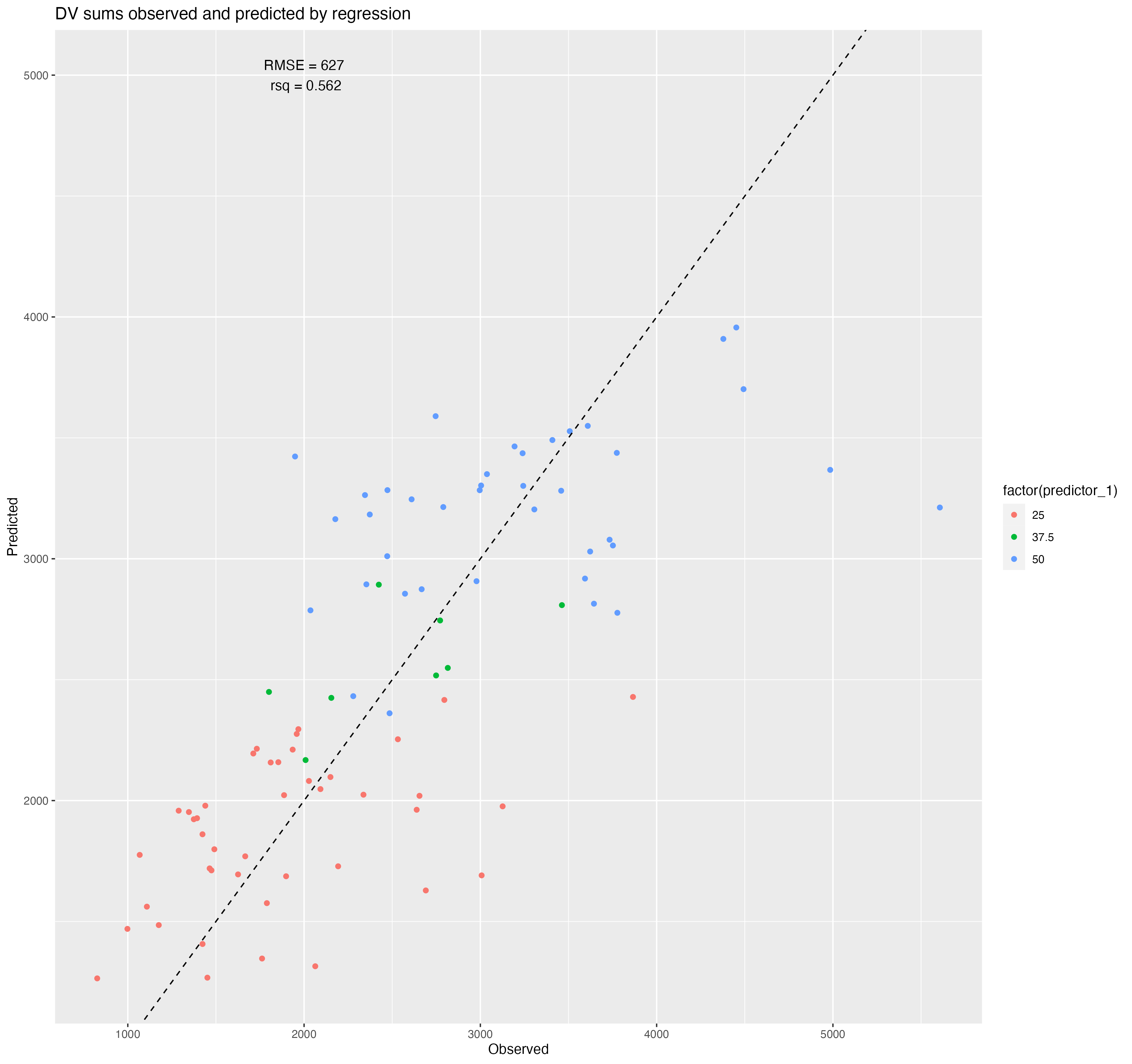
| .metric | .estimator | .estimate |
|---|---|---|
| rmse | standard | 627.4407539 |
| rsq | standard | 0.5622706 |
We compare the RMSE of the above two regression models to the RMSE of a null model predicting the mean y for each observation without considering DOSE.
#null model
null_y_reg = null_model() %>%
  set_engine("parsnip") %>%
  set_mode("regression") %>%
  translate()

null_model = fit(null_y_reg, formula = y ~ 1, data = training)

# calculate r^2 and RMSE from y_DOSE_reg model
## make predictions based on real DOSE observations
predictions_null_model = data.frame(predictor = training$DOSE,
                                    .pred = predict(null_model, new_data = training %>% select(-y)), #use regression model to make y predictions from existing DOSE observations
                                    observation = training$y) #bind to observed y observations

## lets take a look
plot = ggplot() + geom_point(data = predictions_null_model, aes(x = predictor, y = observation, color = factor(predictor))) +
          geom_point(data = predictions_y_DOSE_reg, aes(x = predictor, y = .pred)) +
          geom_line(data = predictions_y_DOSE_reg, aes(x = predictor, y = .pred), linetype = "dashed") +
          labs(x = "Dose", y = "DV sum", title = "Null model prediction of DV sum, y")

## now lets calculate our metrics
metrics = yardstick::metric_set(rmse)
table = metrics(predictions_null_model, truth = observation, estimate = .pred)

## add rmse and rsq to plot
plot = plot + annotate("text", y = 4500, x = 32.5, label = paste0("RMSE = ", round(table[1,3], 0)))

# saving outputs
summarytable_file = here("fitting-exercise", "tables", "metrics_null_model.rds")
saveRDS(table, file = summarytable_file)

figure_file = here("fitting-exercise", "figures", "metrics_null_model.png")
ggsave(filename = figure_file, plot=plot) 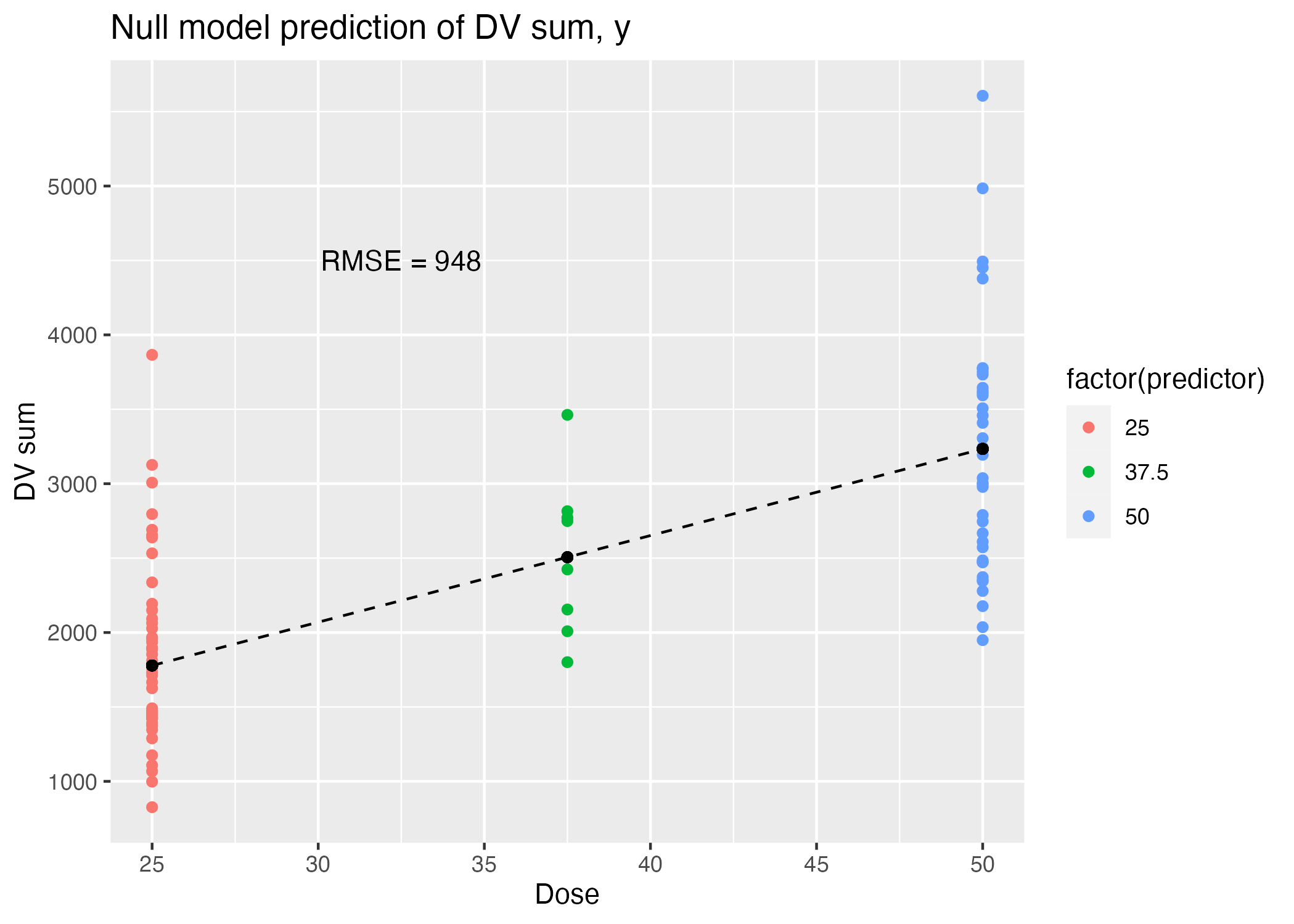
| .metric | .estimator | .estimate |
|---|---|---|
| rmse | standard | 948.3526 |
Comparing the RMSE values reported in Table 9, Table 11, and ?@tbl-metrics-null-model, we can see that the model with the smallest mean roots squared error is the multiple regression model. However, we can also observe that the \(R^2\) value is greater for the single regression model with DOSE as a predictor, which should be taken into consideration when choosing whether the model with a greater number of parameters is truly the “better” model, and not simply the model with the greatest (over?) fit.
Assessing the model performance in a more rigorous way - against unseen data - can improve our understanding of the precision with which the model captures the behavior of the outcome variable based on the predictors. One way to do so is cross-validation.
Cross-Validation of Three Possible Models
In this section, we conduct a 10-fold cross-validation of each model against the training dataset according to the workflow suggest in the Introduction to TidyModels.
The package rsample is used here to create the resampling object - the folds of our data, or indices of random subsets, which will be used in the analysis and assessment of the models.
set.seed(rngseed) #we are resampling randomly, and should set seed for reproducibility

#here, we define the cross-validation folds from our training data
folds = rsample::vfold_cv(training, v = 10) #we would like to define 10 folds
We would like to define two workflow() objects to bundle the two linear model - formula specifications.
####### workflow for single regression of y by dose ########
# choose model with parsnip package
y_DOSE_reg =
  parsnip::linear_reg() %>% #linear regression model
  parsnip::set_engine("lm") %>% #with lm method
  parsnip::set_mode("regression") #mode = regression, mode outcome is numeric

# we can turn this into a workflow with workflows package
y_DOSE_reg_WF =
  workflows::workflow() %>% #defining workflow object
  workflows::add_model(y_DOSE_reg) %>% #choosing the model for the workflow
  workflows::add_formula(y ~ DOSE) %>%
  fit(data = training)

##########################################################################
###### workflow for multiple regression of y by all predictors #######
# choose model with parsnip package
y_multiple_reg =
  parsnip::linear_reg() %>% #linear regression model
  parsnip::set_engine("lm") %>% #with lm method
  parsnip::set_mode("regression") #mode = regression, mode outcome is numeric

# we can turn this into a workflow with workflows package
y_multiple_reg_WF =
  workflows::workflow() %>% #defining workflow object
  workflows::add_model(y_multiple_reg) %>% #choosing the model for the workflow
  workflows::add_formula(y ~ .) %>%
fit(data = training)set.seed(rngseed)
# CV single regression, y ~ DOSE
train_y_dose_rs = y_DOSE_reg_WF %>%
tune::fit_resamples(folds)
train_y_dose_CV_metrics = tune::collect_metrics(train_y_dose_rs) # extract metrics
# CV multiple regression, y ~ all
train_y_multiple_rs = y_multiple_reg_WF %>%
tune::fit_resamples(folds)
train_y_multiple_CV_metrics = tune::collect_metrics(train_y_multiple_rs) # extrac metrics
## CV on null mdoel doesnt make sense, of course, because the mean of the observations will stay the same. I am simply going to re-fit the null model here to keep the RMSE output in one place :)
# refit for null model
null_y_reg = null_model() %>% #fit null model
set_engine("parsnip") %>%
set_mode("regression") %>%
translate()
null_model_metrics = fit(null_y_reg, formula = y ~ 1, data = training) %>% #extract RMSE
predict(new_data = training) %>% #make predictions based on training data
select(.pred) %>% # isolate predicted values
bind_cols(training$y) %>% # bind predictions to training data observations
rename(y = "...2") %>% #rename column containing observations
rmse(truth = y, estimate = .pred) #calculate
#create table with CV output for each model
table1 = cbind("Predictor" = rep(c("DOSE", "multiple"), each = 2), rbind(train_y_dose_CV_metrics, train_y_multiple_CV_metrics)) #table comparing CV of linear regression models
table2 = null_model_metrics
# saving outputs
summarytable_file = here("fitting-exercise", "tables", "metrics_CV_models_training.rds")
saveRDS(table1, file = summarytable_file)
summarytable_file = here("fitting-exercise", "tables", "metrics_null_model_CV.rds")
saveRDS(table2, file = summarytable_file)| Predictor | .metric | .estimator | mean | n | std_err | .config |
|---|---|---|---|---|---|---|
| DOSE | rmse | standard | 690.5397679 | 10 | 67.4950937 | Preprocessor1_Model1 |
| DOSE | rsq | standard | 0.5117853 | 10 | 0.0592077 | Preprocessor1_Model1 |
| multiple | rmse | standard | 645.6909159 | 10 | 64.8192708 | Preprocessor1_Model1 |
| multiple | rsq | standard | 0.5729141 | 10 | 0.0685670 | Preprocessor1_Model1 |
| .metric | .estimator | .estimate |
|---|---|---|
| rmse | standard | 948.3526 |
The mean RMSE of the linear regression model with DOSE as a single predictor has actually improved from 702 to 690, though it is still outperformed by the multiple linear regression model, with a mean RMSE of 645. Here, we also see that the \(R^2\) value of the multiple regression model has improved and also demonstrates a greater fit of the model than the single regression model (though only slightly).
This section added by Cassia Roth
Model Predictions
First, we will put the observed values and the predicted values from the 3 original model fits to all of the training data (the ones without the CV) into a data frame as well as adding a label to indicate the model. Then we will use ggplot to create a figure that plots as symbols observed values on the x-axis and predictions from each of the 3 models, including the null model on the y-axis. I have used a different color and/or a different symbol to differentiate between the 3 model predictions. Both x and y axes go from 0 to 5000 and include a 45 degree line.
# ChatGPT and Taylor Glass's example helped me with this code.

# Create data frame with the observed values and predicted values
plotdata <- data.frame(
  observed = training$y,
  predicted_model1 = predictions_y_DOSE_reg_train$.pred,
  predicted_model2 = predictions_y_multiple_reg_train$.pred,  # Adding predicted values from the second model
  predicted_null = predictions_null_model$.pred,  # Adding predicted values from the null model
  model = c(rep("model 1", nrow(training)),  # Adding labels for each model
            rep("model 2", nrow(training)),
            rep("null model", nrow(training)))
)
plotdata
observed predicted_model1 predicted_model2 predicted_null model
1 3004.21 3206.650 3303.028 2509.171 model 1
2 1346.62 1871.052 1952.556 2509.171 model 1
3 2771.69 2538.851 2744.878 2509.171 model 1
4 2027.60 1871.052 2081.182 2509.171 model 1
5 2353.40 3206.650 2894.205 2509.171 model 1
6 826.43 1871.052 1264.763 2509.171 model 1
7 3865.79 1871.052 2428.627 2509.171 model 1
8 3126.37 1871.052 1976.185 2509.171 model 1
9 1108.17 1871.052 1561.336 2509.171 model 1
10 2815.26 2538.851 2548.685 2509.171 model 1
11 1788.89 1871.052 1575.912 2509.171 model 1
12 1374.48 1871.052 1922.814 2509.171 model 1
13 2485.00 3206.650 2361.116 2509.171 model 1
14 3458.43 3206.650 3281.325 2509.171 model 1
15 1439.57 1871.052 1978.826 2509.171 model 1
16 2532.10 1871.052 2253.618 2509.171 model 1
17 1948.80 3206.650 3422.975 2509.171 model 1
18 2978.20 3206.650 2907.248 2509.171 model 1
19 1800.79 2538.851 2449.336 2509.171 model 1
20 2610.00 3206.650 3245.884 2509.171 model 1
21 4451.84 3206.650 3956.416 2509.171 model 1
22 3306.15 3206.650 3204.047 2509.171 model 1
23 1451.50 1871.052 1267.688 2509.171 model 1
24 3462.59 2538.851 2808.324 2509.171 model 1
25 2177.20 3206.650 3163.879 2509.171 model 1
26 3751.90 3206.650 3054.970 2509.171 model 1
27 2278.97 3206.650 2431.811 2509.171 model 1
28 1175.69 1871.052 1485.125 2509.171 model 1
29 1490.93 1871.052 1798.728 2509.171 model 1
30 1886.48 1871.052 2022.501 2509.171 model 1
31 3777.20 3206.650 2776.584 2509.171 model 1
32 3609.33 3206.650 3549.538 2509.171 model 1
33 2654.70 1871.052 2019.776 2509.171 model 1
34 2063.43 1871.052 1314.893 2509.171 model 1
35 2149.61 1871.052 2097.371 2509.171 model 1
36 2193.20 1871.052 1728.261 2509.171 model 1
37 2372.70 3206.650 3183.098 2509.171 model 1
38 4493.01 3206.650 3701.456 2509.171 model 1
39 1810.59 1871.052 2157.603 2509.171 model 1
40 1666.10 1871.052 1769.537 2509.171 model 1
41 2638.81 1871.052 1962.071 2509.171 model 1
42 1731.80 1871.052 2214.390 2509.171 model 1
43 1423.70 1871.052 1860.657 2509.171 model 1
44 4378.37 3206.650 3909.195 2509.171 model 1
45 3243.29 3206.650 3301.437 2509.171 model 1
46 3774.00 3206.650 3437.942 2509.171 model 1
47 2336.89 1871.052 2024.359 2509.171 model 1
48 1712.00 1871.052 2194.708 2509.171 model 1
49 3239.66 3206.650 3436.449 2509.171 model 1
50 3193.98 3206.650 3464.606 2509.171 model 1
51 2795.65 1871.052 2416.191 2509.171 model 1
52 2572.45 3206.650 2855.525 2509.171 model 1
53 2008.52 2538.851 2167.618 2509.171 model 1
54 3507.10 3206.650 3527.530 2509.171 model 1
55 1958.27 1871.052 2275.623 2509.171 model 1
56 1898.00 1871.052 1687.029 2509.171 model 1
57 3644.37 3206.650 2814.220 2509.171 model 1
58 2092.89 1871.052 2047.547 2509.171 model 1
59 2472.90 3206.650 3283.833 2509.171 model 1
60 1288.64 1871.052 1958.242 2509.171 model 1
61 3733.10 3206.650 3078.806 2509.171 model 1
62 1392.78 1871.052 1927.145 2509.171 model 1
63 1761.62 1871.052 1346.855 2509.171 model 1
64 3037.39 3206.650 3350.018 2509.171 model 1
65 1474.60 1871.052 1711.456 2509.171 model 1
66 2345.50 3206.650 3263.395 2509.171 model 1
67 4984.57 3206.650 3367.617 2509.171 model 1
68 997.89 1871.052 1469.488 2509.171 model 1
69 2748.86 2538.851 2517.525 2509.171 model 1
70 1853.91 1871.052 2158.730 2509.171 model 1
71 2036.20 3206.650 2786.723 2509.171 model 1
72 2423.89 2538.851 2892.948 2509.171 model 1
73 1935.24 1871.052 2210.778 2509.171 model 1
74 2154.56 2538.851 2424.827 2509.171 model 1
75 1464.29 1871.052 1719.560 2509.171 model 1
76 3007.20 1871.052 1690.728 2509.171 model 1
77 3622.80 3206.650 3029.952 2509.171 model 1
78 2789.70 3206.650 3213.928 2509.171 model 1
79 1424.00 1871.052 1406.861 2509.171 model 1
80 2667.02 3206.650 2874.060 2509.171 model 1
81 1967.61 1871.052 2295.337 2509.171 model 1
82 2471.60 3206.650 3010.616 2509.171 model 1
83 2690.52 1871.052 1628.400 2509.171 model 1
84 2746.20 3206.650 3589.721 2509.171 model 1
85 3593.55 3206.650 2918.086 2509.171 model 1
86 1625.46 1871.052 1694.713 2509.171 model 1
87 1067.56 1871.052 1775.419 2509.171 model 1
88 5606.58 3206.650 3211.962 2509.171 model 1
89 3408.61 3206.650 3490.975 2509.171 model 1
90 2996.40 3206.650 3283.515 2509.171 model 1
91 3004.21 3206.650 3303.028 2509.171 model 2
92 1346.62 1871.052 1952.556 2509.171 model 2
93 2771.69 2538.851 2744.878 2509.171 model 2
94 2027.60 1871.052 2081.182 2509.171 model 2
95 2353.40 3206.650 2894.205 2509.171 model 2
96 826.43 1871.052 1264.763 2509.171 model 2
97 3865.79 1871.052 2428.627 2509.171 model 2
98 3126.37 1871.052 1976.185 2509.171 model 2
99 1108.17 1871.052 1561.336 2509.171 model 2
100 2815.26 2538.851 2548.685 2509.171 model 2
101 1788.89 1871.052 1575.912 2509.171 model 2
102 1374.48 1871.052 1922.814 2509.171 model 2
103 2485.00 3206.650 2361.116 2509.171 model 2
104 3458.43 3206.650 3281.325 2509.171 model 2
105 1439.57 1871.052 1978.826 2509.171 model 2
106 2532.10 1871.052 2253.618 2509.171 model 2
107 1948.80 3206.650 3422.975 2509.171 model 2
108 2978.20 3206.650 2907.248 2509.171 model 2
109 1800.79 2538.851 2449.336 2509.171 model 2
110 2610.00 3206.650 3245.884 2509.171 model 2
111 4451.84 3206.650 3956.416 2509.171 model 2
112 3306.15 3206.650 3204.047 2509.171 model 2
113 1451.50 1871.052 1267.688 2509.171 model 2
114 3462.59 2538.851 2808.324 2509.171 model 2
115 2177.20 3206.650 3163.879 2509.171 model 2
116 3751.90 3206.650 3054.970 2509.171 model 2
117 2278.97 3206.650 2431.811 2509.171 model 2
118 1175.69 1871.052 1485.125 2509.171 model 2
119 1490.93 1871.052 1798.728 2509.171 model 2
120 1886.48 1871.052 2022.501 2509.171 model 2
121 3777.20 3206.650 2776.584 2509.171 model 2
122 3609.33 3206.650 3549.538 2509.171 model 2
123 2654.70 1871.052 2019.776 2509.171 model 2
124 2063.43 1871.052 1314.893 2509.171 model 2
125 2149.61 1871.052 2097.371 2509.171 model 2
126 2193.20 1871.052 1728.261 2509.171 model 2
127 2372.70 3206.650 3183.098 2509.171 model 2
128 4493.01 3206.650 3701.456 2509.171 model 2
129 1810.59 1871.052 2157.603 2509.171 model 2
130 1666.10 1871.052 1769.537 2509.171 model 2
131 2638.81 1871.052 1962.071 2509.171 model 2
132 1731.80 1871.052 2214.390 2509.171 model 2
133 1423.70 1871.052 1860.657 2509.171 model 2
134 4378.37 3206.650 3909.195 2509.171 model 2
135 3243.29 3206.650 3301.437 2509.171 model 2
136 3774.00 3206.650 3437.942 2509.171 model 2
137 2336.89 1871.052 2024.359 2509.171 model 2
138 1712.00 1871.052 2194.708 2509.171 model 2
139 3239.66 3206.650 3436.449 2509.171 model 2
140 3193.98 3206.650 3464.606 2509.171 model 2
141 2795.65 1871.052 2416.191 2509.171 model 2
142 2572.45 3206.650 2855.525 2509.171 model 2
143 2008.52 2538.851 2167.618 2509.171 model 2
144 3507.10 3206.650 3527.530 2509.171 model 2
145 1958.27 1871.052 2275.623 2509.171 model 2
146 1898.00 1871.052 1687.029 2509.171 model 2
147 3644.37 3206.650 2814.220 2509.171 model 2
148 2092.89 1871.052 2047.547 2509.171 model 2
149 2472.90 3206.650 3283.833 2509.171 model 2
150 1288.64 1871.052 1958.242 2509.171 model 2
151 3733.10 3206.650 3078.806 2509.171 model 2
152 1392.78 1871.052 1927.145 2509.171 model 2
153 1761.62 1871.052 1346.855 2509.171 model 2
154 3037.39 3206.650 3350.018 2509.171 model 2
155 1474.60 1871.052 1711.456 2509.171 model 2
156 2345.50 3206.650 3263.395 2509.171 model 2
157 4984.57 3206.650 3367.617 2509.171 model 2
158 997.89 1871.052 1469.488 2509.171 model 2
159 2748.86 2538.851 2517.525 2509.171 model 2
160 1853.91 1871.052 2158.730 2509.171 model 2
161 2036.20 3206.650 2786.723 2509.171 model 2
162 2423.89 2538.851 2892.948 2509.171 model 2
163 1935.24 1871.052 2210.778 2509.171 model 2
164 2154.56 2538.851 2424.827 2509.171 model 2
165 1464.29 1871.052 1719.560 2509.171 model 2
166 3007.20 1871.052 1690.728 2509.171 model 2
167 3622.80 3206.650 3029.952 2509.171 model 2
168 2789.70 3206.650 3213.928 2509.171 model 2
169 1424.00 1871.052 1406.861 2509.171 model 2
170 2667.02 3206.650 2874.060 2509.171 model 2
171 1967.61 1871.052 2295.337 2509.171 model 2
172 2471.60 3206.650 3010.616 2509.171 model 2
173 2690.52 1871.052 1628.400 2509.171 model 2
174 2746.20 3206.650 3589.721 2509.171 model 2
175 3593.55 3206.650 2918.086 2509.171 model 2
176 1625.46 1871.052 1694.713 2509.171 model 2
177 1067.56 1871.052 1775.419 2509.171 model 2
178 5606.58 3206.650 3211.962 2509.171 model 2
179 3408.61 3206.650 3490.975 2509.171 model 2
180 2996.40 3206.650 3283.515 2509.171 model 2
181 3004.21 3206.650 3303.028 2509.171 null model
182 1346.62 1871.052 1952.556 2509.171 null model
183 2771.69 2538.851 2744.878 2509.171 null model
184 2027.60 1871.052 2081.182 2509.171 null model
185 2353.40 3206.650 2894.205 2509.171 null model
186 826.43 1871.052 1264.763 2509.171 null model
187 3865.79 1871.052 2428.627 2509.171 null model
188 3126.37 1871.052 1976.185 2509.171 null model
189 1108.17 1871.052 1561.336 2509.171 null model
190 2815.26 2538.851 2548.685 2509.171 null model
191 1788.89 1871.052 1575.912 2509.171 null model
192 1374.48 1871.052 1922.814 2509.171 null model
193 2485.00 3206.650 2361.116 2509.171 null model
194 3458.43 3206.650 3281.325 2509.171 null model
195 1439.57 1871.052 1978.826 2509.171 null model
196 2532.10 1871.052 2253.618 2509.171 null model
197 1948.80 3206.650 3422.975 2509.171 null model
198 2978.20 3206.650 2907.248 2509.171 null model
199 1800.79 2538.851 2449.336 2509.171 null model
200 2610.00 3206.650 3245.884 2509.171 null model
201 4451.84 3206.650 3956.416 2509.171 null model
202 3306.15 3206.650 3204.047 2509.171 null model
203 1451.50 1871.052 1267.688 2509.171 null model
204 3462.59 2538.851 2808.324 2509.171 null model
205 2177.20 3206.650 3163.879 2509.171 null model
206 3751.90 3206.650 3054.970 2509.171 null model
207 2278.97 3206.650 2431.811 2509.171 null model
208 1175.69 1871.052 1485.125 2509.171 null model
209 1490.93 1871.052 1798.728 2509.171 null model
210 1886.48 1871.052 2022.501 2509.171 null model
211 3777.20 3206.650 2776.584 2509.171 null model
212 3609.33 3206.650 3549.538 2509.171 null model
213 2654.70 1871.052 2019.776 2509.171 null model
214 2063.43 1871.052 1314.893 2509.171 null model
215 2149.61 1871.052 2097.371 2509.171 null model
216 2193.20 1871.052 1728.261 2509.171 null model
217 2372.70 3206.650 3183.098 2509.171 null model
218 4493.01 3206.650 3701.456 2509.171 null model
219 1810.59 1871.052 2157.603 2509.171 null model
220 1666.10 1871.052 1769.537 2509.171 null model
221 2638.81 1871.052 1962.071 2509.171 null model
222 1731.80 1871.052 2214.390 2509.171 null model
223 1423.70 1871.052 1860.657 2509.171 null model
224 4378.37 3206.650 3909.195 2509.171 null model
225 3243.29 3206.650 3301.437 2509.171 null model
226 3774.00 3206.650 3437.942 2509.171 null model
227 2336.89 1871.052 2024.359 2509.171 null model
228 1712.00 1871.052 2194.708 2509.171 null model
229 3239.66 3206.650 3436.449 2509.171 null model
230 3193.98 3206.650 3464.606 2509.171 null model
231 2795.65 1871.052 2416.191 2509.171 null model
232 2572.45 3206.650 2855.525 2509.171 null model
233 2008.52 2538.851 2167.618 2509.171 null model
234 3507.10 3206.650 3527.530 2509.171 null model
235 1958.27 1871.052 2275.623 2509.171 null model
236 1898.00 1871.052 1687.029 2509.171 null model
237 3644.37 3206.650 2814.220 2509.171 null model
238 2092.89 1871.052 2047.547 2509.171 null model
239 2472.90 3206.650 3283.833 2509.171 null model
240 1288.64 1871.052 1958.242 2509.171 null model
241 3733.10 3206.650 3078.806 2509.171 null model
242 1392.78 1871.052 1927.145 2509.171 null model
243 1761.62 1871.052 1346.855 2509.171 null model
244 3037.39 3206.650 3350.018 2509.171 null model
245 1474.60 1871.052 1711.456 2509.171 null model
246 2345.50 3206.650 3263.395 2509.171 null model
247 4984.57 3206.650 3367.617 2509.171 null model
248 997.89 1871.052 1469.488 2509.171 null model
249 2748.86 2538.851 2517.525 2509.171 null model
250 1853.91 1871.052 2158.730 2509.171 null model
251 2036.20 3206.650 2786.723 2509.171 null model
252 2423.89 2538.851 2892.948 2509.171 null model
253 1935.24 1871.052 2210.778 2509.171 null model
254 2154.56 2538.851 2424.827 2509.171 null model
255 1464.29 1871.052 1719.560 2509.171 null model
256 3007.20 1871.052 1690.728 2509.171 null model
257 3622.80 3206.650 3029.952 2509.171 null model
258 2789.70 3206.650 3213.928 2509.171 null model
259 1424.00 1871.052 1406.861 2509.171 null model
260 2667.02 3206.650 2874.060 2509.171 null model
261 1967.61 1871.052 2295.337 2509.171 null model
262 2471.60 3206.650 3010.616 2509.171 null model
263 2690.52 1871.052 1628.400 2509.171 null model
264 2746.20 3206.650 3589.721 2509.171 null model
265 3593.55 3206.650 2918.086 2509.171 null model
266 1625.46 1871.052 1694.713 2509.171 null model
267 1067.56 1871.052 1775.419 2509.171 null model
268 5606.58 3206.650 3211.962 2509.171 null model
269 3408.61 3206.650 3490.975 2509.171 null model
270 2996.40 3206.650 3283.515 2509.171 null model# Use GGplot to create a visual representation
plotmodels <- ggplot(plotdata, aes(x = observed)) +
geom_point(aes(y = predicted_null, color = "null model"), shape = 1) +
geom_point(aes(y = predicted_model1, color = "model 1"), shape = 2) +
geom_point(aes(y = predicted_model2, color = "model 2"), shape = 3) +
geom_abline(slope = 1, intercept = 0, linetype = "dashed", color = "black") + #add the 45 degree line
xlim(0, 5000) + #limit the x-axis values
ylim(0, 5000) + #limit the y-axis values
labs(x = "Observed Values", y = "Predicted Values")
plotmodels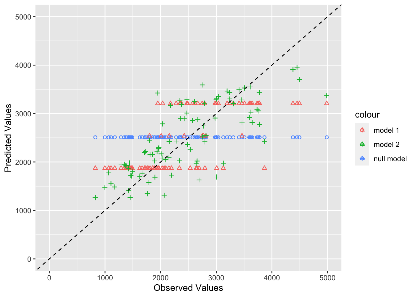
# Save Figure
figure_file = here("fitting-exercise", "figures", "plot_models.png")
ggsave(filename = figure_file, plot=plotmodels) 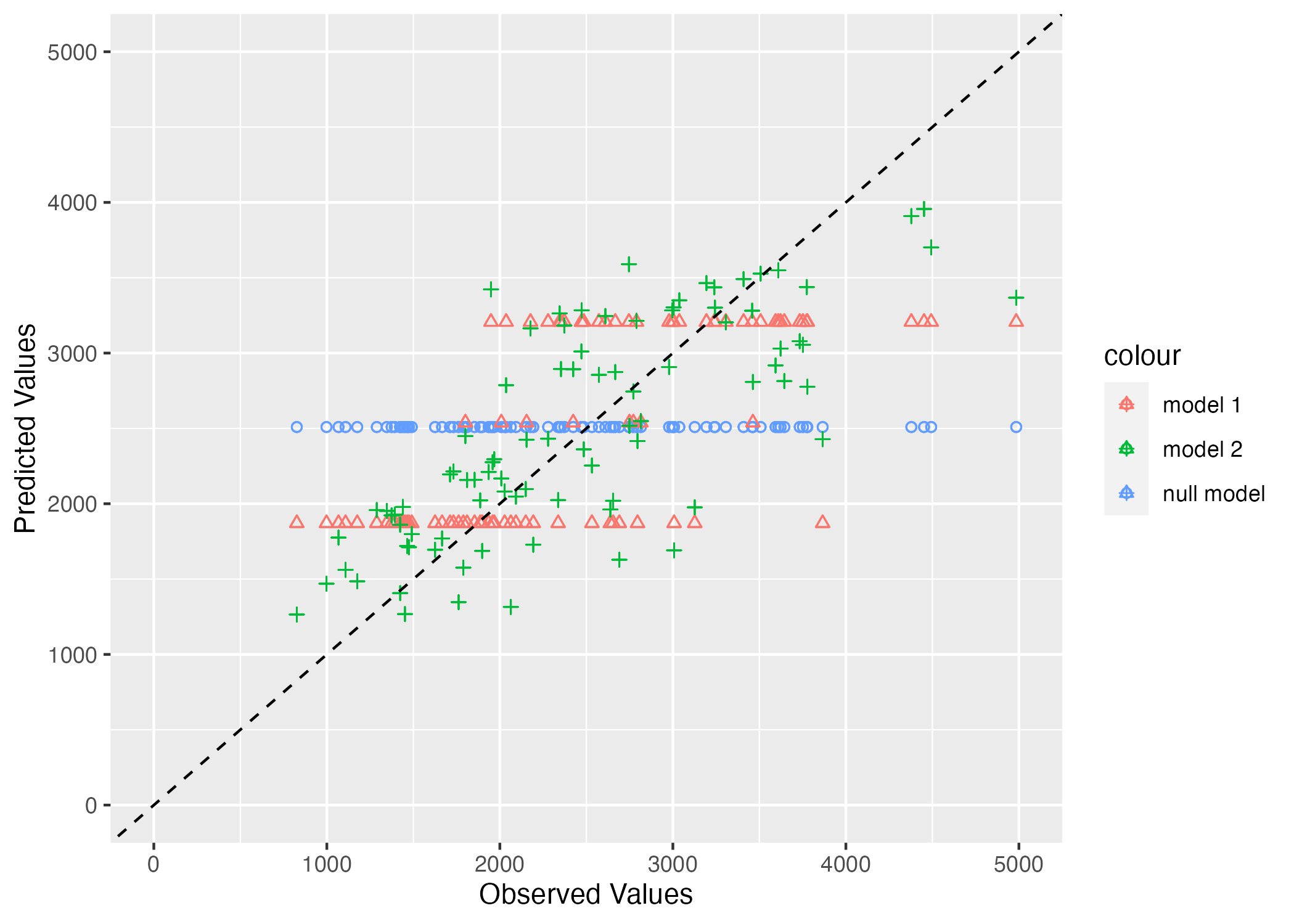
Per Dr. Handel, a good model will have points that fall along the dotted line, showing that observed and predicted values agree – with some scatter. Here we can see that the null model (circles in blue) fall along a horizontal line. This makes sense since they are the mean observations. Model 1 (in red triangles), which only predicts Y based on the DOSE variable falls on three horizontal lines, which corresponds with the variables three discrete values. Finally, the full model, Model 2 (in green plus marks) have more scatter and fall closer to the 45 degree line. This suggests that it is better at predicting the observed values than both the null model and Model 1, the simplest model.
To see if there are patterns to the scatter, we will plot predicted versus residual values for Model 2.
# ChatGPT helped me with this code.

# Calculate residuals for Model 2
plotresiduals <- data.frame(
  predicted_model2 = plotdata$predicted_model2,  # Predicted values from 'plotdata'
  residuals_model2 = plotdata$predicted_model2 - plotdata$observed  # Calculate residuals: predicted - observed
)

# Create the plot
plotresiduals <- ggplot(plotresiduals, aes(x = predicted_model2, y = residuals_model2)) +
  geom_point() +  # Scatter plot of predicted versus residuals
  geom_hline(yintercept = 0, linetype = "dashed", color = "red") +  # Add a horizontal dashed line at y = 0
  xlim(min(plotresiduals$predicted_model2) - 100, max(plotresiduals$predicted_model2) + 100) +  # Adjust x-axis limits
  ylim(min(plotresiduals$residuals_model2) - 100, max(plotresiduals$residuals_model2) + 100) +  # Adjust y-axis limits to symmetrically cover positive and negative residuals
  labs(x = "Predicted Values (Model 2)", y = "Residuals (Model 2)", title = "Predicted vs Residuals Plot for Model 2")
plotresiduals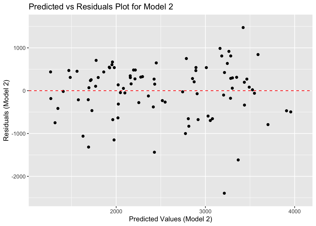
# Save Figure
figure_file = here("fitting-exercise", "figures", "residuals.png")
ggsave(filename = figure_file, plot=plotresiduals)
As Dr. Handel said, a good model will have data in a cloud without any clear pattern. Here, there are more and more negative values compared with positive ones. Thus, our model could be missing something important, or it could still be too simple (imagine if we decided to go with only the DOSE variable)!
Model Predictions and Uncertainty
We have decided we will only focus on Model 2, the more complex linear model, given that it had the best performance from our plotting of the observed versus predicted values.
We will re-set the random seed, using the same values as above. Then, we will use the bootstraps function from the rsample package to create 100 bootstraps, using the training data. Once we store the predictions, we will compute the mean and 89% confidence intervals. Finally, we will plot a figure of observed values on the x-axis and point estimate (obtained from your original predictions on the training data), as well as median and the upper and lower bounds – obtained by the bootstrap sampling and stored in pred on the y-axis. We will use black symbols for the original predictions (the point estimate, or the mean), green to indicate median and blue to indicate lower and upper confidence limits.
# ChatGPT helped me with this code. I also looked at my classmates' Taylor Glass and Emma Hardin-Parker.

# Set seed for reproducibility
set.seed(rngseed)

# create 100 bootstraps with the training data
bootstraps <- bootstraps(training, times = 100)

#creating a list to store predictions from bootstrap training
preds_bootstrap = list()

#Loop through each bootstrap sample
for (i in 1:length(bootstraps$splits)) {
  # Get a single bootstrap sample
  sample_bs <- rsample::analysis(bootstraps$splits[[i]])

  # Fit the model to the current bootstrap sample
  fitted_model <- train_y_multiple_reg_model %>% fit(data = sample_bs)

  #Make predictions for original training data
  predictions <- predict(fitted_model, new_data = training)

  #Store predictions in list
  preds_bootstrap[[i]] <- predictions
}

#Convert list of predictions into a matrix
pred_matrix <- do.call(cbind, preds_bootstrap)

# Compute mean and CIs
preds <- apply(pred_matrix, 1, quantile, c(0.055, 0.5, 0.945))
preds <- t(preds)
preds
5.5% 50% 94.5%
[1,] 3094.7957 3335.818 3546.870
[2,] 1692.3011 1945.359 2165.591
[3,] 2589.7820 2764.634 2931.490
[4,] 1782.8603 2085.856 2384.565
[5,] 2665.4132 2933.091 3137.513
[6,] 1061.3931 1298.528 1484.655
[7,] 2184.4058 2427.685 2641.559
[8,] 1683.2788 1938.921 2294.620
[9,] 1233.9942 1546.862 1881.970
[10,] 2435.0065 2554.059 2714.902
[11,] 1233.1517 1565.327 1891.256
[12,] 1730.7579 1906.337 2150.274
[13,] 1993.2589 2433.874 2755.752
[14,] 2905.6464 3276.160 3607.740
[15,] 1749.0469 2001.055 2246.980
[16,] 2046.5949 2253.406 2466.089
[17,] 3155.1996 3420.669 3742.381
[18,] 2597.0351 2939.237 3242.182
[19,] 2097.1233 2409.333 2849.530
[20,] 3077.3160 3272.769 3511.245
[21,] 3652.3840 3977.786 4250.384
[22,] 3006.3126 3230.275 3511.870
[23,] 962.8575 1269.008 1532.331
[24,] 2362.1508 2804.293 3188.544
[25,] 2958.8739 3195.367 3393.144
[26,] 2795.0407 3101.260 3295.514
[27,] 2065.3904 2496.206 2821.922
[28,] 1334.6525 1506.335 1677.527
[29,] 1579.4553 1798.228 1997.180
[30,] 1614.4527 2002.149 2329.051
[31,] 2589.1124 2823.863 3015.827
[32,] 3380.1637 3561.809 3824.955
[33,] 1801.1927 2024.578 2210.029
[34,] 1140.4386 1321.917 1536.722
[35,] 1877.2462 2108.049 2332.382
[36,] 1569.3843 1712.633 1956.710
[37,] 2905.5287 3215.788 3439.218
[38,] 3349.9890 3717.095 4036.089
[39,] 1945.6153 2176.087 2413.943
[40,] 1406.1824 1760.759 2059.445
[41,] 1803.2971 1970.964 2126.263
[42,] 2049.4052 2220.161 2394.709
[43,] 1646.8191 1857.165 2079.055
[44,] 3709.6352 3919.814 4222.912
[45,] 3095.2887 3341.018 3560.924
[46,] 3060.2967 3459.574 3782.098
[47,] 1823.6533 2041.159 2261.926
[48,] 1993.7931 2204.819 2424.789
[49,] 3256.4765 3470.434 3734.135
[50,] 3218.6991 3473.038 3748.865
[51,] 2230.1721 2425.340 2617.533
[52,] 2613.3955 2895.214 3130.305
[53,] 2017.0420 2172.967 2327.564
[54,] 3358.3423 3550.942 3831.903
[55,] 2082.6792 2278.101 2479.201
[56,] 1533.3173 1699.230 1860.624
[57,] 2597.7486 2872.049 3108.602
[58,] 1684.7083 2017.845 2396.931
[59,] 3045.6565 3309.233 3526.518
[60,] 1781.8228 1975.238 2154.769
[61,] 2911.2546 3109.538 3307.680
[62,] 1640.3969 1907.352 2246.568
[63,] 1129.7014 1372.599 1584.371
[64,] 3212.6261 3372.227 3573.898
[65,] 1473.6308 1706.032 1938.280
[66,] 3006.8834 3276.261 3518.245
[67,] 2995.7371 3368.875 3756.822
[68,] 1276.5988 1467.442 1685.900
[69,] 2266.8108 2502.088 2796.948
[70,] 2001.3116 2167.275 2359.308
[71,] 2412.3821 2849.919 3274.022
[72,] 2669.3929 2902.600 3120.301
[73,] 2055.1219 2220.764 2372.485
[74,] 2294.9412 2437.686 2622.336
[75,] 1548.9537 1729.489 1914.910
[76,] 1499.6668 1703.745 1901.748
[77,] 2852.5998 3070.627 3234.662
[78,] 2882.9232 3156.651 3610.263
[79,] 1123.4597 1383.594 1643.393
[80,] 2589.6832 2865.992 3193.087
[81,] 2102.9400 2316.107 2504.838
[82,] 2750.4584 3061.010 3293.182
[83,] 1409.5569 1629.635 1807.772
[84,] 3229.1419 3611.036 3916.672
[85,] 2648.6181 2957.983 3242.031
[86,] 1564.9562 1708.330 1852.592
[87,] 1599.7097 1787.883 1955.205
[88,] 3033.1130 3243.381 3436.254
[89,] 3199.7180 3487.279 3804.366
[90,] 3133.7900 3315.270 3496.768# create a data frame with all the necessary variables
finaldata <- data.frame(
observed = c(training$y),
point_estimates = c(predictions_y_multiple_reg_train$.pred),
medians = preds[, 2],
lower_bound = preds[, 1],
upper_bound = preds[, 3]
)
# create visualization with all 5 variables
finalplot <- ggplot(finaldata, aes(x = observed, y = point_estimates)) +
geom_point(color = "black") +
geom_point(aes(y = medians), color = "green") +
geom_errorbar(aes(ymin = lower_bound, ymax = upper_bound), width = 0.1, color = "blue") +
geom_abline(slope = 1, intercept = 0, linetype = "dashed", color = "black") + # add 45 degree line
xlim(0, 5000) +
ylim(0, 5000) +
labs(x = "Observed Values", y = "Predicted Values")
finalplot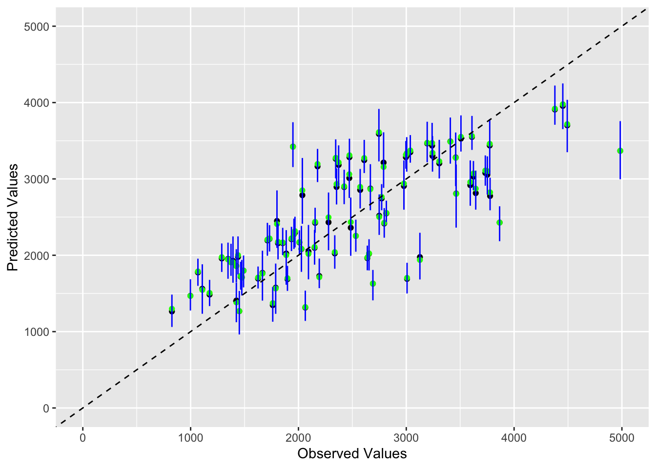
# Save Figure
figure_file = here("fitting-exercise", "figures", "final_plot.png")
ggsave(filename = figure_file, plot=finalplot)
With this plot, we can see that our model does a relatively good job of predicting the observed values. The black points are the original predictions, the green points are the median of the bootstrapped predictions, and the blue lines are the 89% confidence intervals. The 45 degree line is included to show where the observed and predicted values would be if they were the same. Most of the point estimates (the black dots) are very close to the predicted values from the bootstrapping exercise, and both are close to the 45 degree line. Finally, the confidence intervals are relatively narrow. This suggests that our model is doing a good job of predicting the observed values and that we can be relatively confident in our predictions.
Part 3: Final Model Evaluation on Test Data (Cora Hirst)
In this section, we utilize the parameter estimates from the multiple regression model (not acquired from the bootstrapping exercise, but the model fit to the entirety of our training data.) Refer to Table 10.
We will be assessing the performance of this model on our unseen test data, which was earlier stored in the object testing.
# make predictions on testing data
predictions_test <- predict(train_y_multiple_reg_model, new_data = testing)$.pred

#for the sake of keeping everything in one code chunk, I am going to generate my predicitons on the training data again.
predictions_train  = predict(train_y_multiple_reg_model, new_data = training)$.pred

# plot
ggplot() + geom_point(aes(x = testing$y, y = predictions_test, col = "test")) +
  geom_point(aes(x=training$y, y = predictions_train, col = "train")) +
  labs(x = "observed y", y = "predicted y", title = "comparison of performance of trained model on training and test data") +
  geom_abline(linetype = "dashed")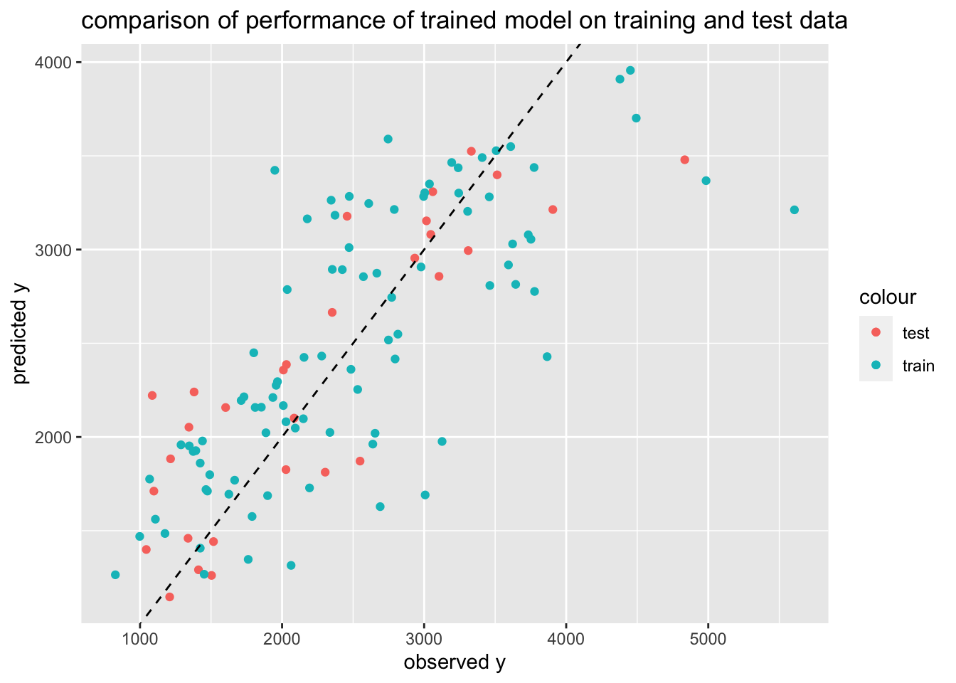
While both the single linear regression model of y by DOSE and the multiple ression of y against all predictor variables fit the data better than the Null Model (Figure 15.) In fact, model 1 - which predicts y based solely on DOSE, appears to predict the “ball park” of where we would expect y to be at that dose. Not considering a person’s height or weight, I’m not sure any real practicioner of drug adminstator would base a person’s dosage solely on this model, but it seems to have a significant effect on y.
Model 2 does further improve results, and this makes sense - not only are we using more observation (person!) specific variables like height and weight to predict a continuous outcome, but also, it appears that we aren’t overfitting the data too terribly.
What I will say is that model 2 does fail to capture a nonlinear increase in y at high y values, that is, large y values are larger than what a linear model with all predictors predicts, and this is clear from the model’s performance on unseen test data, as well. Unless these high y values are biologically relevant and easy to achieve, I’m not sure we need to worry about a more specific, non-linear model to catch this trend. However, if these high y values are potentially dangerous, we may want to identify which variables this nonlinear trend is most correlated with.